I. Introduction
Electricity outage cost (EOC) estimates ($ per kWh unserved) are essential input data for optimal reliability planning and efficient pricing of electricity services (Chao, 1983; Hobbs, 1995; Sreedharan et al., 2012; Wilkerson et al., 2014; Woo et al., 2019, 2023). Compiling reasonable estimates for electricity services’ EOC is complicated due to the diverse EOC estimates reported in literature (e.g., Caves et al., 1990; D. Cheng & Vankatsesh, 2014; Mao et al., 2018; Schröder & Kuckshinrichs, 2015; Woo & Pupp, 1992). Adopting an unrealistically high EOC estimate causes an electric grid to overstate the optimal planning reserve and marginal-cost-based retail price.
Motivated by earlier studies and the large disparity in extant EOC estimates, we used market data from 2019 to 2020 published by two US government agencies to estimate average EOCs of the lower 48 US states. The US Energy Information Administration’s (EIA) market data reflects that 2019 is the most recent pre-Covid year and 2020 is the first year of the Covid pandemic that wrecked the US economy.
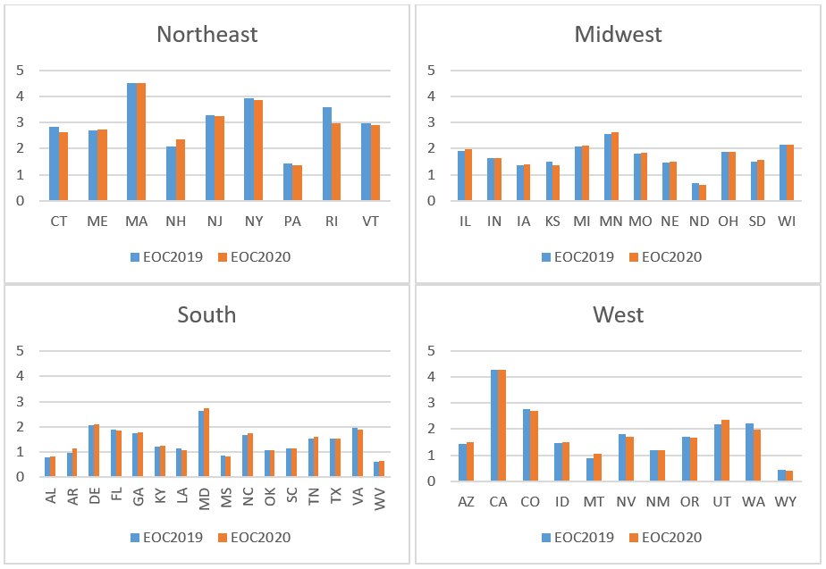
Our main result in Figure 1 shows the market-based EOC estimates by census region and year, leading to the following key findings: First, Figure 1’s median estimates by census region are $1.39 to $2.93 per kWh unserved, far exceeding the residential market-based estimates of $0.12 to $0.34 per kWh unserved (Woo et al., 2021b). However, they are less than the non-residential (commercial and industrial) market-based estimate of ~$3.6 per kWh unserved (Woo et al., 2021a).[1] Second, Figure 1’s median estimates are well below the EOC estimate of $9 per kWh unserved adopted by Texas for the state’s optimal reliability planning (Potomac Economics, 2019) based on the least-cost condition of LOLE × EOC = MGCC, where LOLE = loss-of-load expectation (hours per year) and MGCC = marginal generation capacity cost ($/kW/year) (Chao, 1983; Woo et al., 2019).[2]
This paper is an easy-to-use approach applicable to international regions with similar data availability. Hence, the approach is a quick reality check of the EOC estimates obtained through the more time-consuming approaches like survey-based contingent valuation and choice experiment (e.g., Hartman et al., 1991; Hoyos, 2010; Mitchell & Carson, 1989; Moeltner & Layton, 2002; Ozbafli & Jenkins, 2016; Reichl et al., 2013) and market-based regression analyses of electricity consumption and backup generation ownership (e.g., Y. S. Cheng et al., 2013; Fisher-Vanden et al., 2015; Matsukawa & Fujii, 1994; Tishler, 1993).
The Section II contains the methodology and data, Section III presents the results and the Section IV concludes the paper.
II. Methodology and Data
A. Short-run EOC formula
Our short-run EOC formula is an adaptation of Woo et al.'s (2021b, 2021a) methodology. Consider a state’s cost function for aggregate production:
C = C(Y, P_1, \ldots, P_J, \mathbf{K}, A) = Σ_j P_j X_j \tag{1}
where Y = aggregate output index; Pj = price of input Xj with j = 1 for electricity, 2 for natural gas, 3 for fuel oil, 4 for propane, 5 for labor; K = vector of fixed inputs (e.g., capital and land); and A = total amount of electricity available.
Including an additional input, such as material (e.g., plastic or steel), does not change the EOC formula presented below when the usage of material is strictly proportional to Y (Woo et al., 2021a). This is because the material content of Y in the short-run should not depend on the usage of X1 to X5.
We used max(G, X1) to measure A, where G = annual total generation × (1 – average line loss of 5%). Overlooked by the above cited EOC studies, this measurement of A reflects interstate electricity trading under wholesale market competition in the US (Cao et al., 2021). If a state is an exporter, G > X1, and G measures a state’s total amount of electricity available. If the state is an importer, G < X1, and its electricity import is (X1 – G) > 0, implying that X1 proxies the state’s total amount of electricity available.
Invoking the Envelope Theorem (Takayama, 1985), the effect of ∆A on C is represented as follows:
∆C = Σ_j P_j ∂X_j/∂A ∆A \tag{2}
Let εj = (∂Xj/∂A) (A / Xj) denote the elasticity of Xj with respect to A, which allows us to rewrite equation (2) as:
∆C/∆A = Σ_j ε_j (P_j X_j / A) \tag{3}
We expect εj ≤ 1, as a 1% increase in A raises the usage of Xj by less than 1%. This is because if electricity availability is not a binding constraint in the state’s aggregate production process, the percentage increase in Xj is zero. When the constraint is binding, the percentage increase in Xj is at most equal to 1. As the empirical value of εj is seldom known, we assume εj’s maximum value of 1.0 to obtain the following short-run EOC formula:
EOC = Σ_j P_j X_j / A \tag{4}
B. Data description
The EIA (https://www.eia.gov/electricity/data.php) publishes the state-level data for (a) the prices and total usages by energy type listed in Table 1 and (b) annual electricity consumption and generation for constructing the variable A.
The US Bureau of Labor Statistics (BLS) (www.bls.gov) publishes state-level data for average workhours per week and annual earnings of all nonfarm workers for calculating P5 and X5. Specifically, P5 = E / W, where E is the annual earnings per employee and W is the annual workhours per employee computed as average workhours per week × 52 calendar weeks per year. Further, X5 = N W, where N = total number of nonfarm workers.
III. Results
Table 1 presents the descriptive statistics for {Pj}, {Xj} and A.
The following observations emerge from Table 1. First, electricity prices average $0.11/kWh and exhibit discernible variations based on their standard deviation, coefficient of variation, and minimum and maximum values. Second, the prices for natural gas, fuel oil, and propane have respective averages of $3.75/Mcf, $2.58/gallon and $2.19/gallon with discernible variations. Third, energy and labor usage at the state level are large with notable dispersions. Finally, the average amount of electricity available exceeds the average amount of electricity usage, affirming the US electricity industry’s goal of providing highly reliable service through interstate electricity trading.
Figure 1 presents the EOC estimates by census region and year. These estimates have median values of $1.38 to $2.97 per kWh unserved for 2019 and $1.39 to $2.90 per kWh unserved for 2020, well below the estimate of $9 per kWh unserved as adopted by Texas for optimal reliability planning (Potomac Economics, 2019). Hence, adopting the EOC estimates shown in Figure 1 is likely to reduce the Texas electric grid’s least-cost capacity reserve target of ~13.5% of system peak demand forecast. However, reducing an electric grid’s reserve target is highly controversial, a topic that is well beyond our paper’s narrow focus on EOC estimation.
_estimates_(___per_kwh_unserved)_for_the_lower_48_s.png)
IV. Conclusion
Our paper’s research focus reflects that EOC estimates are essential input data for least-cost resource planning and efficient electricity pricing, and the extant EOC estimates are highly diverse, complicating their use by these applications. Our key findings are as follows: First, our EOC estimates are well below the estimate adopted by Texas for optimal reliability planning. Second, our proposed approach is easy to use with minimal data requirement, thus readily applicable to international regions with market data akin to those published by the EIA and BLS. Hence, it can serve as a quick reality check of EOC estimates obtained through other approaches that are far more time-consuming to implement.
The policy implications of adopting our lower EOC estimates are (a) a reduction in an electric grid’s optimal planning reserve that improves the grid’s cost efficiency; and (b) a decline in the grid’s marginal cost-based retail price that encourages welfare-enhancing end-use consumption. However, (a) and (b) represent a sharp departure from the status quo. Hence, they should be a policy debate topic among the stakeholders of a region’s electricity industry (e.g., Woo et al., 2023).
Funding
This study was partially funded by the Ford Foundation (#134371 and #139746) and the Research Matching Grant Scheme of the Research Grant Council of the HKSAR Government, and supported by Shenzhen Humanities & Social Sciences Key Research Bases.
Acknowledgment
We thank the editors and two reviewers for their helpful comments. Without implications, all errors are ours.
Woo et al.'s (2021b) non-residential estimate was based on an overstated wage of $75 per hour, about three times the correctly stated wage of $27/hour. Using the correct wage of $27/hour, the non-residential EOC estimate should have been ~3.6 per kWh unserved.
Since the optimal LOLE equals MGCC / EOC, a decrease in EOC implies an increase in the optimal LOLE and a reduction in an electric grid’s planning reserve.