Commodity Market Efficiency: New Evidence From the Russia-Ukraine War

I. Introduction

The efficient market hypothesis (EMH), first postulated by Fama (1970), explains how asset prices or financial markets obey the random walk theory before they are deemed fully efficient. EMH can be in the weak-form efficiency, where asset prices adjust to historical information or past trends; the semi-strong form efficiency, in which asset prices adjust to publicly available information; or the strong form efficiency where insider information is already reflected in asset prices, making it practically impossible to beat the market (Fama, 1970). However, crises such as the Global Financial crisis, European sovereign debt crisis, Brexit, and Covid-19 pandemic, present trend price deviation and unexpected investor behaviour, particularly market participants with active portfolios engaging in arbitrage (Moyo et al., 2023; Olowe, 1996). Expecting a comparable pattern during the ongoing Russia-Ukraine war seems admissible. Meanwhile, the commodity market has been historically used as a hedge during crisis periods, especially their futures (Chauhau et al., 2013), due to lesser volatilities to critical periods within these markets. Interestingly, these markets, notably energy markets, are conventionally regarded as efficient markets. Thus, the efficiency of commodity markets before and after the Russia-Ukraine war commencement needs to be assessed. This study examined the agricultural, energy, and metal futures markets, selecting five proxies for each class of commodity market.

Various methodologies have been adopted to evaluate market efficiency. The multifractal detrended fluctuation analysis (Aslam et al., 2022) employed 30-minutes intra-day data; the vector error correction model and Johansen co-integration and granger causality tests (Manogna & Mishra, 2023) analyze the nine most liquid agricultural commodities; and similarly, panel integration was used by Khedhiri (2023) to determine the efficiency of the agricultural commodity market. However, this study adopted the average variance ratio (AVR) test to appraise the efficiency of commodity markets due to its adequacy for testing individual markets’ weak-form efficiency (Charles & Darné, 2009; Smith & Ryoo, 2003) as opposed to testing the overall market efficiency of a market class. Few studies have investigated the impact of the Russia-Ukraine war on market efficiency, and no study has analyzed the selected commodity markets. Therefore, this study examines how the Russia-Ukraine war has affected the commodity markets by comparatively assessing the markets’ efficiency before and after the war’s start. This study provides detailed information for portfolio managers, and hedgers to create effective portfolio baskets and informs policymakers about the areas needing improved regulations in the financial market. We observed that the commodity markets considered were inefficient both before and after the war commenced except gasoline and oats, which became efficient after the war commenced. In addition to this introductory section, the paper is organized as follows: Section II presents the methodology, Section III discusses the findings, and Section IV concludes the paper.

II. Methodology and Data

Variance ratios have been frequently used in testing hypotheses in time series analyses (returns form) (Charles & Darné, 2009). We randomly selected the commodity market proxies, wherein the return series, $X_{t}$ equals $Q_{t}$. The apriori expectation was for the series to follow a martingale difference sequence. In determining this, the following conditions are necessary;

$$E\left( Q_{t} \right) = 0,\ \ \forall\ {'}t{'};\ and\ E\left( Q_{t}Q_{t - k} \right) = 0,\forall\ {'}k{'}.\tag{1}$$

The AVR test mainly sets side by side the variance of the $f - th$ period difference ${\lbrack\widehat{\delta}}^{2}(f)\rbrack$ with the f-times variance of one period difference $\lbrack{\widehat{\delta}}^{2}(1)$] (see equation (2)). The test statistics was thus ordered to check the null hypothesis for the market efficiency:

$$AVR(f) = \ \frac{{\widehat{\delta}}^{2}(f)}{{\widehat{\delta}}^{2}(1)}\tag{2}$$

$$z(f) = \left( AVR(f) - 1 \right)\ {\{\pi^{2}(f)\}}^{- \frac{1}{2}}\tag{3}$$

The scaled variance is ${\widehat{\delta}}^{2}(f) = \ \frac{1}{T_{f}}\sum_{t = 1}^{T}{(r_{t} - f\mu)}^{2}$, and the mean of the return is $\widehat{\mu} = \ \frac{1}{T}\sum_{t = 1}^{T}r_{t}$, which can be defined as $\pi^{2}(f) = \ \sum_{k = 1}^{f - 1}{(\frac{2(f - k)}{f})}^{2}$ . The kernel estimator is depicted as $\delta_{s}$ ; ${\widehat{\delta}}_{k} = \ {\lbrack\frac{\sum_{t = k + 1}^{T}{{(r_{t - k} - \ \widehat{\mu})}^{2}{(r_{t} - \ \widehat{\mu})}^{2}}}{\sum_{t = k + 1}^{T}{(r_{t - k} - \ \widehat{\mu})}^{2}}\rbrack}^{2}$. The specified significant level for the analysis technique is at 1%, 5%, and 10%. The null hypothesis will therefore be rejected if the probability level is lower than the stated significance level.

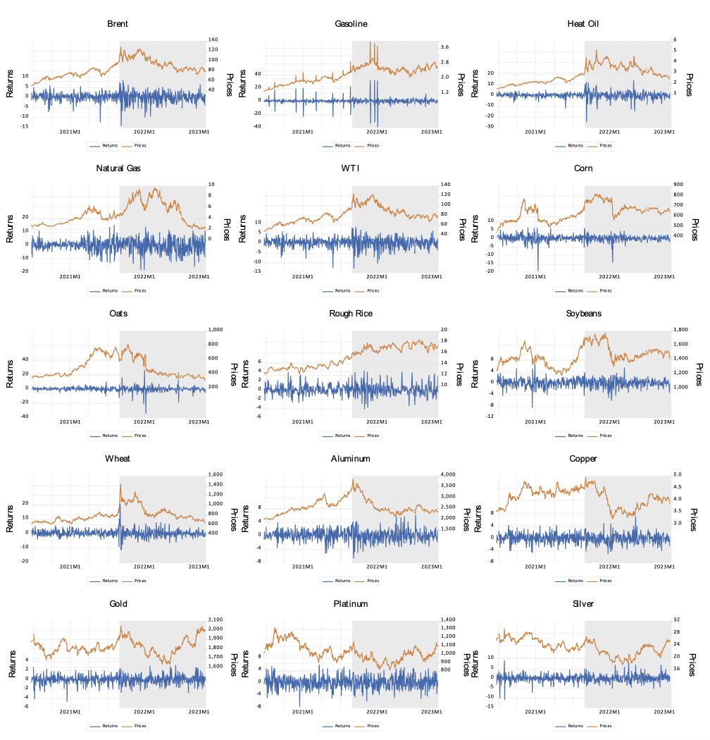
The data set for 608 days was obtained from https://ng.investing.com/currencies/, and a level of analysis was conducted on the returns obtained. The study spanned two major periods, with an equal number of days before and after the war commenced. Preliminary analyses were conducted using exploratory tools on the futures raw prices and returns for each commodity price’s data series (Figure 1). Remarkable differences in the prices and returns were observed before and after the start of the war.

The descriptive data analysis of the variables showed that WTI had the highest return, while silver had the lowest return before the inception of the war, and rough rice had the maximum return while platinum had the minimum return during the war; most importantly, returns have significantly reduced in the war period. The standard deviations for all indices were relatively low portraying the series as not volatile. In contrast, during the war period, commodities have become more volatile excluding corn and soybeans, whose volatility has reduced with similar results from the coefficient of variation. The observed kurtoses were all leptokurtic except wheat before the war, which had outliers. However, during the war, only platinum followed a normal distribution pattern, while most of the commodities such as Brent, heating oil, natural gas, WTI, corn, soybean, gold, platinum, and silver had a decline in kurtosis. The rest of the commodities, namely gasoline, oats, rough rice, wheat, aluminium, and copper had increased kurtosis. The ARCH tests revealed that quite a number of the series did not exhibit significant conditional heteroskedasticity before the war. However, after the inception of the war, all series except platinum and silver showed a significant heteroskedasticity effect. The correlation statistics also showed no significant change between the pre-war and in-war periods.^[1]

Figure 1.Prices and Returns of Selected Commodities

III. Results

Individual and joint variance ratios were applied to each series within the data set. The holding periods considered were 22, 66, and 132 to represent 1-month, 3-month, and 6-month holding periods respectively. The results for the joint variance ratio tests show that across the three sub-samples, markets are weak-form inefficient before and after the commencement of the war besides gasoline and oats whose market became weak-form efficient during the war. An in-depth analysis of selected holding periods was conducted, and mixed results were obtained. At the 1-month holding period, the markets were weak-form inefficient, and investors could profit from the market. However, there was a disparity in the market efficiency as the holding period extended. At the 3-month holding period, the market efficiency results were mixed: before the war, only corn and oats became weak-form efficient, but three months after the war commenced, gasoline, corn, oats, and wheat became efficient. Ultimately, at the 6-month holding period, all markets became efficient, which implies that lower profit may be achieved for a portfolio basket with such a time lag. Thus, short-term investments would be more profitable in these markets irrespective of the existence or non-existence of a crisis.

IV. Conclusion

This study centres on how the Russia-Ukraine war could have influenced the weak-form efficiency of selected commodity markets. A comparative analysis of before and after the war’s inception was conducted using the conventional average variance ratio method. It was observed that the Russia-Ukraine war has had little or no effect on the weak-form efficiency of the commodity markets. This may be because the markets were inefficient before the inception of the war, which is similar to Aslam et al.'s (2022) findings. Aslam et al. observed market inefficiencies for all energy commodity markets except natural gas, which became more efficient after the commencement of the Russia-Ukraine war. Arguably, past information regarding commodity pricing has not been fully incorporated into current commodity prices, hence the weak-form EMH, opening the markets up to potential arbitrage. Investors could exploit the inefficiencies to achieve profitable investment strategies that deviate from efficiency, providing an arbitrage gain. We implore policymakers and regulators to ensure market efficiency by ensuring public disclosure of all relevant information and strict compliance with market regulations. The same should implement a communication platform for rapid dissemination of information to improve market efficiency.

Acknowledgement

The authors benefitted immensely from the capacity development training programmes at the Centre for Econometrics and Applied Research, Ibadan. Nigeria. The authors are grateful to Dr Ahamuefula. E. Ogbonna and Dr Idris. A. Adediran for helpful comments that led to the successful completion of this work.