
I. Introduction
Evidence-based investment decisions are crucial, as studies reveal a contemporary time frequency link between climate risk and oil stock (Chien et al., 2021; Lorente et al., 2023). In this study, we add to the body of empirical evidence regarding the time frequency relationship between climate risk and oil stock.
Hypothetically, the stock channel relies on the portfolio diversification theory, which predicts an inverse linear relationship between climate risk and returns. Climate risk causes incremental demand for climate-related investment at the detriment of conventional stocks including oil stock (Salisu et al., 2023; Tumala et al., 2023). Thus, oil prices plummet due to stock market counter-shocks following net-zero transitions with attendant slow growth, macroeconomic volatility, and weakening external and fiscal positions (Fofack, 2015). Meanwhile, the oil sector’s production process and market fundamentals, including crude oil supply, demand, and prices, are particularly vulnerable to climate risk (He & Zhang, 2022).
This study considers sectoral stock returns, specifically oil-sector stock since investors are susceptible to varying sentiments that influence their demand for stocks. Moreover, stock prices vary across different sectors (Zhou, 2018). Second, the study uses the climate policy uncertainty (CPU) index as a proxy for climate risk. The CPU index, created by Gavriilidis (2021), is a news-based indicator of climate uncertainty.
This study’s crux is the application of the wavelet transformation to examine the association between oil price and climate risk. Wavelet methodology captures idiosyncrasies along time domain and different measuring scales (Haven et al., 2012). Studies have used time-domain methodology to analyse relationships in financial markets (Li et al., 2015; Sousa et al., 2014). These connections, however, may differ among frequencies and evolve with time. Our approach unearths previously undiscovered economic time-frequency relationships. This maiden technique is employed to uncover climate risk-oil stock attributes from 1987 to 2022. These periods accounted for the oil glut, financial crises, COVID-19, and other global downturns. This study promotes understanding the variable of interest, oil prices and climate risks, using refined methodology and providing a global context-specific time-frequency nexus.
The remainder of this paper is structured as follows: Section II provides the data and methodology; Section III deals with empirical results; and the conclusion is detailed in Section IV.
II. Data and Methodology
The study employed monthly data from April 1987 to July 2022. Monthly data is relevant for investigating contagion effects, as shock transmission is swift and rapidly reverts to normalcy. We selected the price of West Texas Intermediate (WTI) crude as a benchmark for establishing the price of other light crudes globally because it is closely tied to other crude oil markets (Wu & Zhu, 2019). WTI prices were retrieved from the investing.com website (https://www.investing.com/), while the dataset for climate policy uncertainty was based on the index developed by Gavriilidis (2021).[1]
Given its effectiveness in examining multi-resolution characteristics, the continuous wavelet transform was used for our analysis. The continuous wavelet transforms (CWT) analyses a definite wavelet against the time sequence and is represented as follows:
Wx(m,n)=∫∞−∞x(t)i√n¯ψ(t−mN)dt
Where
x(t)=1Cψ∫∞0[∫∞−∞Wx(m,n)ψm,n(t)du]dnN2,N>0
Meanwhile, the CWT has the time sequence power observed as:
‖x‖2=1Cψ∫∞0[∫∞−∞|Wx(m,n)|2dm]dnN2
In tandem with the risk-return hypothesis, this study specified the climate risk and oil-stock nexus as follows:
ψ(WTI,CPU)(t,σ)=∫∞−∞WT(WTI)[τ+t,σ]WT(CPU)[τ,σ]∗dτ
Where * denotes the complex conjugate, t, which means the point in a time series with restricted observations where wavelet is applied; σ is the scaling or dilation factor; and τ is the location parameter. CPU is the climate policy uncertainty proxy of climate risks, and WTI measures the oil stock price.
III. Empirical Analyses
A. Wavelet Decomposition
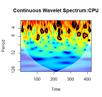
There are many periods in the datasets, and the short- and long-run periods alone do not represent the appropriate time scales in the detailed analysis (Raza et al., 2017). The continuous wavelet power spectrum shows the movement of the series – WTI and CPU – in a three-dimensional contour plot: time, frequency, and color code. The time displayed on the horizontal axis is divided into five: 0 - 100, 101 - 200, 201 - 300, 301 - 400 and 401 - 423 for 1987M04 - 1995M08, 1995M09 - 2004M01, 2004M02 - 2012M06, 2012M07 - 2020M11, 2020M12 -2022M07, respectively. Meanwhile, the vertical axis represents the period such that (0-8), (8-32), (32-64), and (64-128) indicate short-run, medium-run, long-run and very long-run periods, respectively. In Figures 1 and 2, items inside the U area, hereafter cone of influence (COI), are interpreted as the region showing the statistical significance of the series variability. Furthermore, the red regions signal high variability, while the blue depicts area(s) with low variability in the series. The black line represents the 5% significance level; thus, the areas inside the cone contain dynamic patterns which are statistically significant at 95%. All the areas outside the cone are out of consideration, as yellow explains the lower version of red.
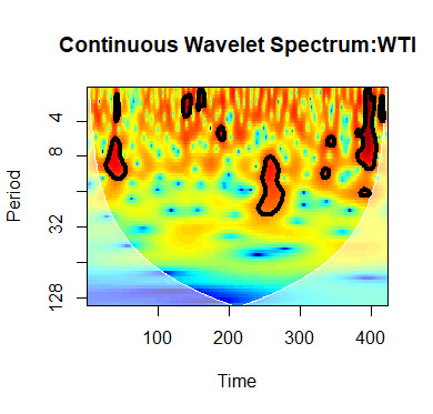
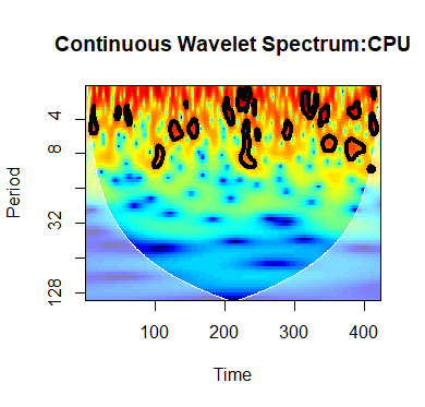
In Figures 1 and 2, at the beginning of the short-run frequency for WTI and CPU, there were deep red areas in 1987, indicating extremely high variability, which was sustained till the early medium-run period. Meanwhile, black shows the series is significant at 5%. The series witnessed a slight appearance of yellow at the beginning of this period, which paved the way for its variance; before long run, volatility was witnessed in August 1995, though mixed with a few blue traces. In Figure 1, from September 1995 to January 2004, the series experienced high variability amidst drifts and spikes in the early short run during the earlier months until later in the medium run. This is contrary to happenings in the CPU series. During the aforementioned months, the CPU series witnessed high variability early in the medium-run frequency and started reversing to the short-run frequency in June 1999, and subsequently witnessed medium-run frequencies in 2002 before the appearance of blue and yellow, signaling low and lower variability respectively, till the end of the time phase.
Further examination revealed the disappearance of the red color at higher frequencies in both figures. However, red (low variability) is more pronounced in Figure 2, with traces of blue signaling shifts into a low variability region. Only the WTI showed high variability in the medium-run frequency during the 201–300 time phase, and it was significant at the 5% level. In contrast, the short-run period was dampened with the yellow color, suggesting that the WTI initially had low variability during the short run but got stronger in the medium run. Only blue areas were identified later in the medium-, long- and very long-run frequencies in Figure 1, implying the absence of co-movements across time scales for the whole sample period. In Figure 2, strong red laden with the black contour represents a significantly high variability of WTI in the short and medium runs.
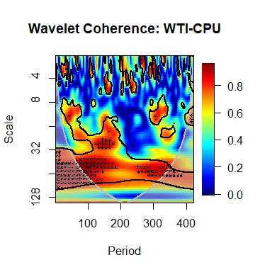
B. Wavelet Transform Coherence
The wavelet coherence was used to establish the lead-lag effect of two variables. It explicitly displayed how variables cross and cause others in frequency bands and intervals, strengthening and revealing the causality between WTI and CPU.
The COI specifies the region with edge effects and is displayed outside the black line. The color code for coherence ranges from blue (low) to red (high). The arrows indicate the phase difference between the two series. Arrows pointing to the right mean that the variable is in phase. Arrows pointing to the left suggest that the variables are out of phase. In-phase indicates that the variables have cyclical effects, and out-of-phase or anti-phase connotes anti-cyclical effects on each other.
Figure 3 exposed that in the short-run period between a 0-100 months cycle, i.e., from 1987M04-1995M08, the arrows were right up, indicating that the variables were exhibiting in-phase effects with WTI leading and CPU lagging, implying that in the short-run period of 1987M04-1995M08, there is a cyclical effect of WTI on CPU. During the period 1995M07–1996M11 (101–200), the arrows pointed left and left down, meaning the variables were out-phase, with CPU lagging and WTI leading in an anti-cyclical effect. Meanwhile, in the 201-300 months cycles short-run period, the arrows pointed left up, indicating out-phase nexus, with CPU leading and WTI lagging, indicating CPU had an anti-cyclical effect on WTI. However, in the early times of 301-400, the arrows turned right down, reflecting in-phase, with CPU leading and WTI lagging and establishing that CPU causes WTI cyclically. Whereas, from 401-423, there is no evidence of short-term causality between the variables.

According to Figure 3, in the medium run (8-32) period, for 0–100-month cycles, the latter time – towards the end of 1993 – witnessed left down arrows indicating out-phase association, with WTI leading and CPU lagging. This means that WTI has a cyclical impact on the CPU during these months. In the subsequent month cycles – 101-200 – we have both left down and right down arrows reflecting out- and in-phase, respectively, with CPU leading and lagging simultaneously in the medium-run period. This attests to the imbalances in CPU globally, which might impact oil stock in some parts of the world and vice versa. There is an overlap from one month cycles to another between 201-300 and 301-400, as the black contour with arrows pointing left down overlaps with the two sets of monthly cycles (see Figure 3). Eventually, the anti-cyclical impact of WTI on CPU occurred towards the end of June 2012 till July 2012. Meanwhile, there are no medium-run effects between WTI and CPU, as there was no evidence of causality between the variables.
The long-run period (32-64) for 0-100 has arrows pointing both left towards the tail end of 1995M08. This indicates an out-phase scenario, meaning WTI leads, creating an anti-cyclical causality on the CPU. The anti-phase effect of the WTI on the CPU was maintained in the succeeding month cycles (101-200), as WTI maintained its out-phase impact on the CPU, which was sustained till early 2012. Finally, the long-run (64-128) period occurred only in 101-200 and 201-300 months, which was abrupt. The long-run impacts favor WTI in an out-phase manner in the two different month cycles. WTI was leading while CPU was lagging, depicting that in some months in 1995M04-2004M01 and 2004M02-2012M06, WTI had a very long-run causal effect on CPU, ceteris paribus.
IV. Conclusion
While most empirical work has investigated climate policy uncertainty and oil-stock nexus over a single time scale, we employed wavelets to analyze this dependence over multiple periods. This methodological framework is capable of detecting variations in climate risk-oil stock relationships during diverse time frames. The results of continuous wavelet power spectra identified the patterns of strong variance in many small, medium, and long periods for oil stock price, while high variance is visible on small and medium scales but is absent during long periods for the CPU. The study established evidence of common variation through the wavelet coherence from 2002 to 2012, wherein long-scale evidence of strong coherence exists between the series in the long-run periods. The results also support the existence of bidirectional causality in the long-run timescale. The study can help investors and policymakers to track the co-movement of climate risk and oil stock. This research can also be used to examine oil-stock fluctuations induced by climate risk and develop strategies for stabilizing the market.
The methodology follows the work of Baker et al. (2016), searching eight leading US newspapers containing the terms {“uncertainty” or “uncertain”} and {“carbon dioxide” or “climate” or “climate risk” or “greenhouse gas emissions” or “greenhouse” or “CO2” or “emissions” or “global warming” or “climate change” or “green energy” or “renewable energy” or “environmental”} and (“regulation” or “legislation” or “White House” or “Congress” or “EPA” or “law” or “policy”} (including variants such as “uncertainties,” “regulatory,” “policies,” etc.).