I. Introduction

In resource-endowed countries, the ability of governments to spend on the critical sectors of their economies depends on the stability of resource prices. Similarly, in crude oil-endowed countries, governments face fiscal constraints during a decline in crude oil prices. Such declines often affect economic performance and mostly result in economic downturns (Raifu et al., 2020). This has been the experience of Nigeria, the largest oil-producing country in Africa. Since crude oil was discovered in 1956 at the Oloibiri village of Niger Delta and became commercialised in the early 1970s, it has become the mainstay of Nigeria’s economy. The survival of Nigeria’s economy largely depends on oil price stability and oil revenue generation.

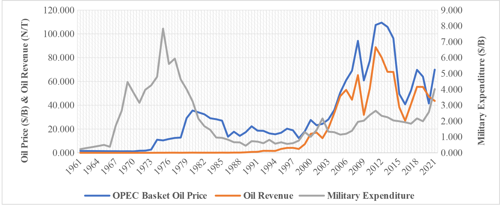
Over the years, data from Nigeria has shown that when oil prices decline, oil revenue and various components of government expenditures, including military expenditure, decline. Figure 1 shows the relationship between military expenditure, oil price and oil revenue in Nigeria over time. It is evident that when oil prices increased, particularly around the 1970s, oil revenue and military expenditure rose in pari-passu and vice versa when oil prices declined. Thus, oil price determines oil revenue realisation, which in turn determines the amount of funds the government can devote to military expenditure (Raifu et al., 2021).

Figure 1 shows the evolution of oil price, oil revenue and military expenditure (1961-2020)

The literature suggests several determinants of military expenditure including gross domestic product (GDP), population, trade openness, political regime, socio-political conflicts, insurgency or insecurity, population of armed forces, existence of external threats, military expenditure of potential enemies and total expenditure on the real enemies (Coutts et al., 2019; Dizaji, 2019; Markowski et al., 2017). Recently, researchers have focused on how oil price shocks affect military expenditure in oil-resource-endowed countries (Bakirtas & Akpolat, 2020; Erdoğan et al., 2020). These studies, however, examine how military expenditure responds to an exogenous change in oil prices without considering the factors that contribute to oil price shocks. For instance, Erdoğan et al. (2020) examined the response of military expenditure to oil price volatility in six Gulf Cooperation Council Countries (United Arab Emirates, Bahrain, Qatar, Kuwait, Saudi Arabia, and Oman). Bakirtas & Akpolat (2020) also investigated the direction of causality among oil exports, oil prices and military expenditure in some Organization of the Petroleum Exporting Countries. This study digresses from the two studies to examine whether the sources of price shocks also determine military expenditure in Nigeria. This study is important because adverse oil shocks could hamper the government’s drive to combat numerous security threats facing the country which require military intervention. We, therefore, hypothesise that oil shocks do not have any significant effect on military expenditure. To affirm our hypothesis, we follow Kilian’s (2009) argument by investigating, apart from the effect of oil price shocks, the effects of two types of oil shocks – demand shocks and oil supply shocks – on military expenditure in Nigeria. To factor in the asymmetric relationship between the shocks and military expenditure, this study used non-linear autoregressive distributed lags (NARDL) proposed by Shin et al. (2014).

Section II presents the methodological approach and data sources. The results are presented in Section III while Section IV concludes.

II. Methodology and Data Sources

This study models the effects of oil shocks (oil price shock, demand shock and supply shock) on military expenditure in Nigeria. Military expenditure was measured in USD million. The military expenditure was obtained from the Stockholm International Peace Research Institute. The nominal Brent crude oil (NBCO) was sourced from the World Bank commodities database. From the NBCO, real BCO (RBCO) was computed using the following formula: $\left(R B C O=\frac{N B C O}{U S C P I} * 100\right)$. The US Consumer Price Index was obtained from the St. Louis FED database. Oil supply and oil demand shocks were obtained from Baumeister and Hamilton (2019). We controlled for other variables such as real GDP per capita, trade openness, and population growth. These variables were obtained from the World Development Indicators (WDI). Other variables include political regime and insecurity, which are dummy variables. Regarding the political regime, the military regime was assigned ‘0’ while the civilian regime was assigned ‘1’. In terms of insecurity, we used 2009 when Boko Haram became a security threat to delineate the period of insecurity and the period of relative peace. So, the period before 2009 was assigned ‘0’ while the period afterwards was assigned ‘1’. We used annual data from 1976 to 2021.

We began the specification of NARDL from the long-run model which shows the effects of oil shocks and other variables on military expenditure.

$$m i l s_t=\alpha_0+\alpha_1 o i l s_t^{+}+\alpha_1 \text { oils } s_t^{-}+\alpha^{\prime} X_t+\varepsilon_t \tag{1}$$

Following Shin et al. (2014), oil shocks can be decomposed into a partial sum of positive and negative components as follows:

$$\begin{aligned} &\text { oils } s_t^{+}=\sum_{j=1}^t \Delta o i l s_t^{+}=\sum_{j=1}^t \max \left(\Delta o i l s_j, 0\right) ; \\& \text { oils } s_t^{-}=\sum_{j=1}^t \Delta o i l s_t^{-}=\sum_{j=1}^t \min \left(\Delta o i l s_j, 0\right) \end{aligned}\tag{2}$$

$$\begin{aligned} \Delta m i l s_t=&\alpha_0+\alpha_1 o i l s_t^{+}+\alpha_2 o i l s_t^{-}+\alpha^{\prime} X_t\\&+\sum_{j=1}^p \beta_j \Delta m i l s_{t-1}\\&+\sum_{j=0}^q\left(\beta_t^{+} \Delta o i l s_{t-1}^{+}+\beta_t^{-} \Delta o i l s_{t-1}^{-}\right)\\&+\sum_{j=0}^t \beta_t^{\prime} \Delta X_{t-1}+\varepsilon_t \end{aligned} \tag{3}$$

Where $mils$ is military expenditure, $oils$ is the oil shocks (+ and -), $X$ represents other variables such as GDP per capita, population growth, trade openness, political regime (military regime or civilian regime) and insecurity; $p$, $q$ and $t$ are the lags order, $\alpha$’s are the long-run coefficients while $\beta$’s are the short-run coefficients. However, the coefficients of the short-run asymmetric distributed lags are $\sum_{j=0}^q \beta_t^{+}$ and $\sum_{j=0}^q \beta_t^{-}$ for positive and negative oil shocks respectively. The long-run positive and negative effects of oil shocks can be represented as: $\delta_1^{+}=\frac{\alpha_1^{+}}{\alpha_0}$ and $\delta_2^{-}=\frac{\alpha_2^{-}}{\alpha_0}$ respectively. The null hypothesis of the long effect of oil shocks is given as $p=\delta_t^{+}=\delta_t^{-}=0$ while the null hypothesis of the short run is $\sum_{j=0}^q \beta_t^{+}=\sum_{j=0}^q \beta_t^{-}$. The error correction model for the NARDL model is specified as follows:

$$\begin{aligned} \Delta \text { mils }=&\alpha_0+\sum_{j=0}^q\left(\beta_t^{+} \Delta o i l s_{t-1}^{+}+\beta_t^{-} \Delta o i l s_{t-1}^{-}\right)\\&+\sum_{j=0}^t \beta_t^{\prime} \Delta X_{t-1}+\lambda e c t_{t-1}+\varepsilon_t\end{aligned} \tag{4}$$

Where $e c t_{t-1}$ denotes the error correction term and $\lambda$ is the coefficient of the error correction term.

Before implementing the ARDL model, we performed the Phillips-Perron unit root on the variables mentioned above to ensure that none of the variables is integrated of order 2. This is because the results of bounds testing would be spurious if any of the variables is integrated of order 2. Even though the lag lengths vary across the models, the Akaike Information Criterion was used to select the lag lengths with the aid of the internal iteration mechanism of EVIEW software.

III. Empirical Results

Before the NARDL analysis, we conducted some preliminary tests such as the descriptive analysis and unit root test. We only reported the results of the unit root test in Table 1.^[1] As shown in the table, none of the variables is integrated of order 2. The variables are a mixture of integration of orders 0 and 1, that is, they are I(0) and I(1).

Table 2 reports the results of NARDL. As previously stated, we considered the effect of oil price shock (model 1), oil demand shock (model 2) and oil supply shock (model 3). In all three models, there is evidence of cointegration among the variables, suggesting the existence of a long-run relationship because the F-bounds statistics are greater than the upper bounds criteria. This is corroborated by the results of error correction models (ECM). The ECM’s results showed that there is an adjustment towards the long-run equilibrium if there is a short-run disequilibrium in the system (except in model 2 when the ECM estimate is -1.791). We also confirmed the existence of both short-run and long-run asymmetries in all the three models.

In model 1, a positive shock to the oil price by 1% increases military expenditure by 1.430% while a negative shock to the oil price shock by 1% reduces military expenditure by 0.572% in the short run. In the long run, even though both positive and negative shocks to oil prices lead to positive growth in military expenditure, only a negative shock is statistically significant at 10%. Our findings are in tandem with those of Erdoğan, et al (2020). Model 2 provides evidence that positive and negative shocks to the demand for crude oil lead to an increase (0.031%) and decrease (0.074%) in military expenditure in the short run while in model 3, positive and negative shocks to oil supply lead to a decline (0.154%) and increase (0.931%) in military expenditure in the short run respectively. These findings support the a priori expectation from the theory of demand and supply. An increase in demand for crude oil would lead to an increase in crude oil prices which in turn brings about an increase in oil revenue accrued to the government. An increase in oil revenue signifies that more funds are available for the government to spend on different sectors of the economy. In the long run, however, both positive and negative shocks to the demand for and supply of crude oil lead to a reduction in military expenditure in models 2 and 3. We also find that the post-estimation diagnostic results are reliable in all the three models.

Briefly, our findings (model 1) show that real GDP per capita increases military expenditure in the short and long run. Population growth reduces military expenditure over time. However, trade openness and the political regime have mixed effects on military expenditure, which is negative in the short run but positive in the long run. Insecurity has a positive effect on military expenditure in the short run but with a lag (2).

IV. Conclusion

Evidence from this study has shown that oil shocks, either in terms of oil price, oil demand or oil supply impact the expenditure on military activities in Nigeria. A negative development in the oil market is detrimental to military expenditure and, thus, it is expedient for the government to design a mechanism for the management of oil revenue, which depends on the vagary of events in the international oil market. Even though the Nigerian government created the Excess Crude Account (ECA) in 2004, the management of the account becomes an albatross, hence, management must be prioritized. The current study is limited to the asymmetric effect of oil shocks on military expenditure in one of the oil-producing countries, and its findings cannot be generalised to other oil-producing countries. Hence, future research can be extended to other countries. Also, factors which affect the relationship between oil shocks and military expenditure should be examined.