I. Introduction

One of the biggest threats to human existence is in the risk inherent in changing climatic conditions.^[1] Climate change has been estimated to have various effects on different aspects of human existence: from the effects it has on air quality (Jacob & Winner, 2009), to the effects it has on the economy (Tol, 2009), its effects on water resources (Barnett et al., 2004), and various aspects of human health (Haines & Patz, 2004).

Efforts to mitigate the adverse effects of climate change have given rise to commitments like the Kyoto Protocol of 1997 and the Paris Agreement of 2015.^[2] Despite these climate agreements, policies around mitigating the negative effects of climate change have not been consistent (for example, the back-and-forth of the United States on the Paris Agreement between Presidents Trump and Biden); meanwhile, global mean temperature has been steadily rising, with the top seven warmest years occurring starting 2015.^[3] This rising temperature and uncertainty in climate policy may be indicative of continued inconsistencies in climate policy, and persistence in global warming measures.

Therefore, it is important to test the time series properties of both climate policy and global warming measures, especially concerning their persistence or otherwise. We test persistence in climate policy uncertainty index (cpu_index)^[4] developed by Gavriilidis (2021), which accounts for attitudes towards climate policy, and persistence in Global Land and Ocean Temperature Anomalies (GLOT)^[5], which measures actual climate change – the departure of global temperature from a long-term average and constructed from land and sea surface temperatures. The GLOT is included in this study given that temperature is likely the most important climatic variable (Strangeways, 2010).^[6] Persistence in cpu_index means climate policy remains uncertain (such as the back-and-forth of the US to stay or leave the Paris Climate Agreement). Persistence in GLOT means temperature anomalies continue to rise above a desired long-term average. What persistence in both measures entails is that attitudes or policies towards reducing global warming may be inconsistent, which may account for increased risk from the adverse effects of global warming.

There are various attempts in literature to test persistence in climate-related issues. For example, the effect of COVID-19 on the transitory nature of CO₂ emissions in the world’s largest emitters shows low level of persistence in CO₂ emissions (Claudio-quiroga & Gil-Alaña, 2022). In Bermejo et al. (2021), atmospheric pollution (suspended particles (PM2.5) and Ozone (O3)) in ten US cities are found to be transitory (low persistence), the same result is obtained for four mega-cities in China (Chen et al., 2016). Meanwhile, temperature has long memory and may lead to future climate warming in Sub-Sahara Africa (Gil-Alaña et al., 2019). Additionally, heterogeneous degrees of persistence in temperature and precipitation exist in US cities (Gil-Alaña et al., 2022). Finally, evidence shows that fine particulate matter (PM_2.5) possesses low persistence implying mean reversion and transitory effect of shocks in 20 megacities across the world (Bermejo et al., 2022).

In this paper, we test for persistence in both cpu_index and GLOT, which represent attitudes towards climate policy and actual change in global climate temperature, respectively. Previous studies are either specific to specific locations or analyze specific climatic indicators. Understanding persistence in these climate change measures will help guide the direction of policies related to climate risk.

We report that the measures have high persistence but are mean reverting. Thus, we establish that actions that are lax on climate change policy, including climate temperature change may last into the future.

II. Methodology

After a shock, if a series tends to slowly return to its equilibrium level, we say that the series has persistence. Since the standard framework^[7] only allows integer degrees of differentiation, our modeling strategy relies on the concept of fractional integration to characterize persistence. For this reason, fractionally integrated methods have gained traction, with an array of empirical applications (Baillie & Bollerslev, 1994; Caporale et al., 2018; Gil-Alaña et al., 2019; Gil-Alaña & Monge, 2020; Gil-Alaña & Robinson, 1997). A more recent theoretical rationale, in terms of shock length (using an error-duration model), has been established, building on the work of Granger and Joyeux (1980).

Granger and Joyeux (1980) introduced the autoregressive fractionally integrated moving average model, which allows for the modeling of persistence or long memory d, where d is a differencing or memory parameter. Therefore, a time series $x_{t}$ follows a fractional process if:

$$\phi(L)(1 - L)^{d}\left( x_{t} - \mu \right) = \Theta(L)\varepsilon_{t}\tag{1}$$

where, $\phi(L)$ and $\Theta(L)$ are the autoregressive and moving average polynomials, respectively; $L$ is the backward-shift operator and $\varepsilon_{t}\sim iid(o,\sigma_{\varepsilon}^{2})$. The fractional differencing lag parameter $(1 - L)^{d}$ is expressed by the polynomial expansion:

$$(1 - L)^{d} = \sum_{k = 0}^{\infty}\frac{\Gamma(k - d)L^{k}}{\Gamma( - d)\Gamma(k + 1)}\tag{2}$$

The gamma function is represented by $\Gamma(\blacksquare)$. A fractional process is said to be stationary and invertible when the persistence parameter $d$, $- 0.5 < d < 0.5$. Hence, the autocorrelation function for a zero-integrated process for a such process decays geometrically, while the autocorrelation function for a long-memory process decays hyperbolically, and the autocorrelation coefficients are of the same sign as $d$. To be more specific, when $- 0.5 < d < 0$, since the autocorrelations are negative, we refer to this phenomenon as anti-persistent memory. Secondly, for $0 < d < 0.5$ the process is stationary but has a long memory, and shocks decay hyperbolically rather than geometrically. In addition, when $- 0.5 \leq d < 0.5$ the relevant series in question is non-stationary, with mean reverting tendencies and an unconditional variance growing more slowly than when the persistence parameter$\ d = 1$. Finally, when$\ d \geq 1$ the procedure is characterized as explosive non-mean reverting and non-stationary.

We utilize the maximum likelihood estimator, a parametric method pioneered by Sowell (1992), to estimate the long-memory (fractional integration) parameter, $d$, of a time series. The precision of the parameter estimations generated from the data is a benefit of Sowell (1992).

III. Results

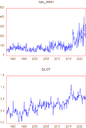
We examine the Gavriilidis (2021) climate policy uncertainty index (cpu_index) and the Global Land and Ocean Temperature Anomalies (GLOT) from the United States National Oceanic and Atmospheric Administration to gauge the persistence in climate risk measures, using available monthly series from April 1987 to August 2022. Our sample period choice stems from the available dataset of the climate policy uncertainty index. The climate uncertainty index is composed of standardized textual data relating to climate risk, greenhouse gas emissions, global warming, and climate change, among others, from eight leading US newspapers. Meanwhile, the GLOT averages both land and ocean temperatures across the globe. Figure 1 below plots the respective series that are used in the analyses. The graph depicts the peaking trend in climate uncertainty, as well as rising global land and ocean temperatures.

Figure 1.Trends in cpu_index and GLOT

Notes: This plot displays the movement in climate policy uncertainty index (cpu_index) and the Global Land and Ocean Temperature Anomalies (GLOT) from April 1987 to August 2022

The estimates of the integration order $d$ in Eq. (1) for the two series in question are shown in Table 1. We show the results under two basic assumptions in the unit root literature: (i) only an intercept or a constant, i.e., with $d = 0$ a priori; and (ii) both an intercept and a (linear) temporal trend, i.e., with both parameters and calculated from the data.

We find that the two series (in Table 1) reflecting climate risk measures have long memory, regardless of whether the model with constant only or the model with constant and trend is used. Specifically, we find significant evidence of persistence in both series, as our persistence parameter, $d$ lies between $0$ and $0.5$. The Wald test statistic is applied to each statistically significant fractional integration parameter to determine the level of long memory inherent in the related series. The Wald test, however, consistently rejects the null hypothesis that the fractional integration parameter is not statistically different from unity. Implicitly, regardless of the sample period or model structure used, all of the series are determined to have long memory and to be mean reverting. As a result, we can conclude that, despite their high persistence, the climate risk indicators are mean reverting. This suggests that the impact of any policy shock will take a long time to dissipate.

We performed a structural break test on the data to ensure its reliability. The Bai and Perron (2003) test, which permits up to five structural breaks in the time series, further supports the necessity of sub-sampling the entire dataset. The break date derived by the Bai-Perron test is October 2016. In light of Table 2 (sub-samples), we investigate the persistence of climate risk indicators. The results presented in Table 2, are not different from those highlighted for the full sample in Table 1. In other words, the climate risk indicators are fractionally integrated, whether the structural break is considered. The persistence found in cpu_index and GLOT is in line with that of Gil-Alana et al. (2019), whereby temperature in Sub-Sahara Africa has long memory, thus leading to future climate warming. The implication of this is that in terms of persistence, the global measure of climate change and climate policy yields results similar to some of the least developed parts of the world, even if persistence is low in more advanced countries (see Bermejo et al., 2021).

IV. Conclusion

In this study, we use the fractional integration method to explore the time series features of climate risk indicators. In addition to characteristics like long-range dependence and persistence, this technique may capture time trend components. Climate change-related risks have far-reaching consequences, and thus have sparked growing concerns and a desire to learn more about them. The widespread effects of climate risks and the growing importance of climate change-related issues inspired our research. We show that the presence of long memory and persistence (even though mean reverting) in cpu_index suggest that policy inactions or uncertainties like the US shifting position on the Paris Agreement may be long-lasting. In addition, persistence in GLOT (which eventually reverts to its mean) suggests that global temperature will continue to rise unless there are policies to mitigate its effects and reduce its risk. Therefore, policymakers, especially from the large emitting countries must reduce climate policy uncertainties, so that the effect of global warming can be mitigated.