I. Introduction

The discovery of the first modern oil in the Russian empire in 1846 has ignited additional and continued oil discoveries across the globe. Oil deposits stood at 15.8 billion barrels in 2019 and are estimated at 4.7 billion barrels in 2021 (Sonnichsen, 2022). Available statistics show that the production of global crude oil has increased more steadily since the year 2000, and it stood at about 4.2 billion metric tons in 2021 but peaked around 2018 to about 4.5 billion metric tons (Sonnichsen, 2022). The oil and gas sector remains one of the important sectors in the global economy valued at US$5 trillion in 2022. Putting these together, additional energy demand surge across the globe together with existing global imbalances among oil exporters would play a significant role on oil supply shocks across the world. Theory posits that fossil-fuel economic ascension inflicts damages on the environment (see Akadiri et al., 2022; Grossman & Krueger, 1991). However, the theoretical link that Hotelling (1931) provides suggests that the seller’s decision to sell his non-renewable natural resource is due to the time value of money and this would lead to increased consumption that further creates pressure on the environment.

There are several empirical studies in the oil shocks and climate change literature, albeit not without serious methodological debates. Prominently, empirical studies employ vector autoregressive-typed techniques to extract the shock components of oil for empirical analyses (see Zhao, 2020). Killian (2009) employ a two-staged decoupling method of structural vector autoregression and a few authors use the same approach. Authors in this category include He and Zhou (2018), Gupta et al. (2021), Zhao (2020), Azhgaliyeva et al. (2022), Mohammed et al. (2022), among others. The major setback of the Killian (2009) method is its indecisiveness in separating respective oil shocks (see Ready, 2018). Consequent upon this shortfall, many researchers (see Anand & Paul, 2021; Ready, 2018) made efforts to recalibrate and augment the standard two-staged structural vector autoregression model of Killian (2009). Other authors, including Naeem et al. (2021), Chatziantoniou et al. (2022), Zhang et al. (2022), among others, adopt the variants of these recalibrations. To address the identification issues, Baumeister and Hamilton (2019) provide a Bayesian extension to the Killian (2009) framework, which decomposes the shocks from oil price into four separate components as against the three components advanced in the baseline method. Later authors with the same approach are Huang et al. (2020) and Gupta et al. (2021).

The most popular result from these studies has further reinforced the concreteness of the oil shocks and climate risk debate, necessitating the need for global evidence. In contrasting studies, Guo et al. (2022) employ a time-varying model to show the asymmetric effect of climate policy uncertainty on oil price movements in the Unites States, while Pierdzioch (2021) and Salisu et al. (2022) find that climate risks foster volatilities in the oil market. Despite these strident research efforts, the submission that oil supply shocks contribute to climate risks is still an open debate. This study contributes to the existing literature that seeks to explain the role that carbon-emission activities, through increasing supply of oil to the global economy, play in climate change. This study contributes to the literature in the following significant ways. First, it is the first study to employ the Bergstrand (2019) data to investigate the impact of oil supply shocks on climate risk. Second, this is one of the few studies contributing to the methodological literature by using the Mixed Data Sampling (MIDAS) approach to analyze oil supply series according to their original data generating process.

II. Data and Preliminary Analysis

As highlighted above, the literature documents the measurement issues on oil shocks. However, there is no consensus on the measures of climate risk yet. Two major components of climate risks (physical and transition risks) have been identified.^[1] The former is geared towards news on global warming (GW) and natural disaster (ND) due to physical natural hazards, while the latter relates to those resulting from the uncoordinated transition towards a green economy. Authors have developed indexes for both measures (Faccini et al., 2021, 2022; Penikas, 2022). The measures geared towards GW and ND have enjoyed high patronage for measuring physical climate risks. The adequacy of these indexes has supported its adoption from several studies (see, e.g., Bouri et al., 2022; Gupta & Pierdzioch, 2021; Salisu et al., 2022). This study adopts the computed global warming index following the literature. For the oil supply shocks, the computed index by Baumeister and Hamilton (2019) was adopted. This is a streamline of various identification problems inherent in the VAR-typed models of shock extractions through estimated posterior medians. The data on climate change spans from 2000/01/03 to 2018/12/31, covering 4,780 observations, while the data on oil supply shocks spans the period from January 2000 to December 2018, covering 229 observations.

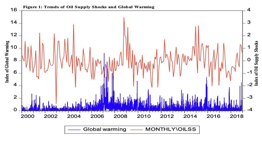
Figure 1 provides the trend analyses on both oil supply shocks and global warming. It is evident from the trends that global warming, before 2006, was relatively moderate but became much pronounced since 2008 (see Figure 1). Figure 2 is highly instructive as it illustrates symbolic shock waves across the periods under consideration. The trend indicates that global oil supply is characterised by intermittent patterns of shocks, and this peaked between 2008 and 2009. This coincides with the period from 2007 to 2009 (i.e., global financial crisis). A deeply negative oil supply shock was noticed around 2002 and there was a noticeable increase since the beginning of 2018. For all other periods, the global oil supply was characterised by a lot of cyclicality (see Figure 1). A similar pattern is noticed with the global warming, which peaked between 12/13/2006 to 01/03/2008 and 9/21//2015 and 3/28/2016 (see Figure 1). The statistical properties of the variables, including the descriptive statistics and tests for heteroscedasticity and autocorrelation, are depicted in Table 1. The mean value for oil supply shocks is -0.055 and this shows that the shocks to oil supply is negative on the average, indicating that supply to the global oil market is more of a reduction than declining supply. On the other hand, the mean value of 0.385 for global warming indicates that it moderately gravitates towards the minimum value of 0.000 than the maximum value of 9.218. This is an indication that global warming challenges could be lower when shocks from oil supply reduce on the average over the period under consideration. However, the 3.878 skewness for global warming and 0.474 for oil supply shocks are positive and mean that oil supply and global warming increases are more common.

 

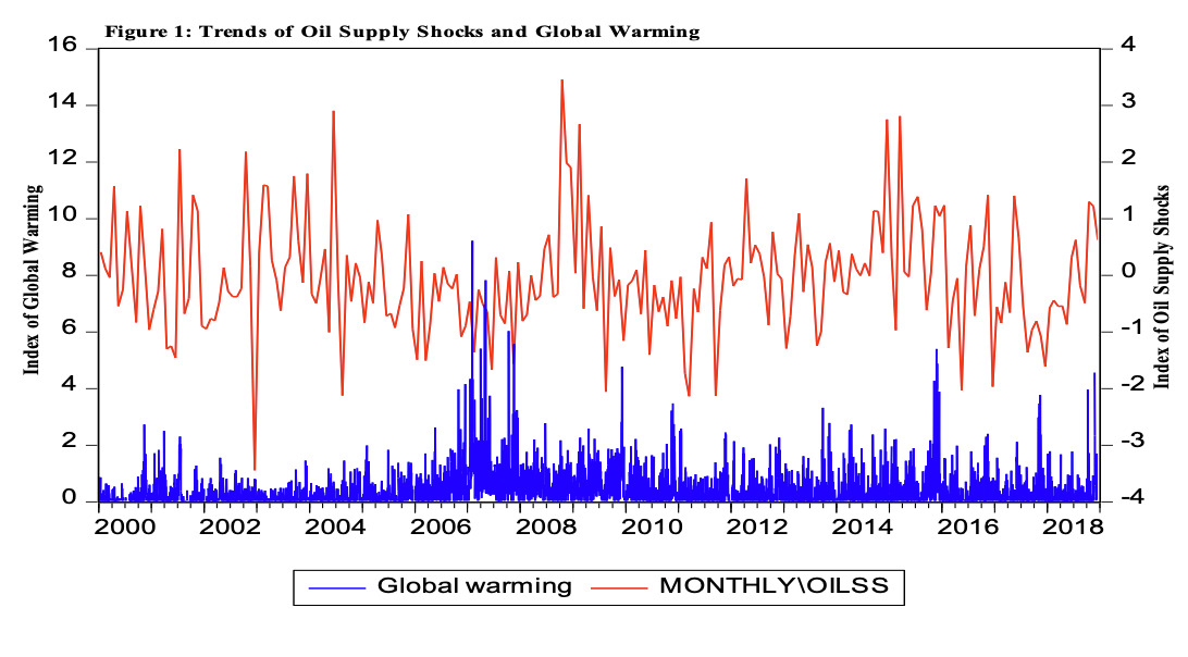
Figure 1 depicts the trends of oil supply shocks and climate risk. The oil supply shocks is the computed index by Baumeister and Hamilton (2019) while the indicator for climate risk is a composite news index on global warming. The former is a monthly data while the latter is a daily data; both spanned the period 2000 – 2018.

The kurtosis values of 4.282 and 31.209 for the respective variables mean that both variables have leptokurtic distributions and are heavy tailed. The Jarque-Bera statistics, as a formal test for normality, reject the null hypothesis that the two series are normally distributed at the 1 percent level of significance (see Panel 1A of Table 1). The ARCH LM test supports the presence of ARCH effects as the null hypothesis that the series are not heteroscedastic is rejected at the 1 percent level at various lag length periods of 2, 4 and 8. Also, the serial correlation test rejects the null hypothesis of no serial correlation at the 1 percent level at the corresponding lag length periods (see Panel B of Table 1). Hence, the most appropriate method of analysis is the ARCH-typed that would inherently include both the serial correlation and heteroscedastic properties of the series into the model.

III. Methodology and Results

A. Theoretical Framework and Model Specifications

The theoretical anchor for oil supply shocks and climate risks harps on the Hotelling (1931) framework. Predicated on the serial correlation and heteroscedasticity tests, the appropriate method of analysis for this study is the ARCH-type method. Consequently, this study employs the Generalized Autoregressive Conditional Heteroscedasticity Mixed Data Sampling (GARCH-MIDAS) approach. Within this framework, the volatility of the global warming index denotes climate risk. This approach is technically desirable as it accommodates variables of different frequencies within the same estimation framework with any extrapolations process that would lead to valuable information loss. In this case, the index of global warming is in daily frequency, while that of the oil supply shocks is in monthly frequency. Given this, the GARCH-MIDAS methodological framework^[2] is as follows.

$$r_{i, t}=\mu+\sqrt{\tau_t \times h_{i, t}} \times \varepsilon_{i, t} \quad \forall i=1, \ldots \ldots \ldots . N_t \tag{1}$$

$$h_{i, t}=(1-\alpha-\beta)+\alpha \frac{\left.r_{i-1, t}-\mu\right)^2}{\tau_i}+\beta \bar{h}_{i-1, t} \tag{2}$$

$$\tau_i^{(r w)}=m_i^{(r w)}+\theta^{(r w)} \sum_{k=1}^K \varphi_k\left(\omega_1 \omega_2\right) X_{i=k}^{(r w)} \tag{3}$$

$$\small{ \varphi_k\left(\omega_1, \omega_2\right)=\frac{[k /(K+1)]^{\omega_1-1} \times[1-k /(K+1)]^{\omega_2-1}}{\sum_{j=1}^K[j /(K+1)]^{\alpha_1-1} \times[1-j /(K+1)]^{\omega_2-1}} } \tag{4}$$

$$\varepsilon_{i, t} \mid \phi_{i-1, t} \sim N(0,1) \tag{5}$$

where $r_{i,t}$ denotes the climate risk measured by the volatility of global warming index; on the $i^{th}$ day of month $t$; $N_t$ denotes the number of days in month $t$; $\mu$ denotes the unconditional mean of the climate risks; $h_{i,t}$ and $\tau$ indicate the short- and long-run components of the conditional variance part of Equation (1). For a model-based volatility behaviour of global warming index, these components are further broken down into Equations (2) and (3), while $h_{i,t}$ (short-run component) adopts a GARCH (1, 1) process, where $\alpha$ and $\beta$ in Equation (2) refer to the ARCH and GARCH terms. The first-order condition for the ARCH and GARCH terms is $\alpha\ > \ 0$, $\beta\ \geq \ 0$ and $\alpha\ + \ \beta\ < \ 1$.

The long-term component $\tau_i$ is initially varying monthly, it is structured to daily frequency as specified in Equation (3); $m$ is the long-run constant, while $\theta$ is slope coefficient (i.e., the sum of weighted rolling window exogenous variable). The parameter $\theta$ shows the impact of oil supply shocks (proxied by OILSS) on the long-run return volatility of stock market. The parameter $\varphi_k\left(\omega_1 \omega_2\right)$ is the beta polynomial weighing scheme, with $\varphi_k\left(\omega_1 \omega_2\right) \geq 0, k=1, \ldots, K$ and summing up to unity for model identification, $X_{i=k}$ represents the predictor variable ($OILSS$), the superscript “rw” implies that the rolling window framework is utilized; and the random shock $\varepsilon_{i, t}$, which is conditional on $\phi_{i-1, t}$ is normally distributed, where $\phi_{i-1, t}$ represents the information set that is available at $i - 1$ day of month $t$. In addition to testing the global impact of oil supply shocks on climate risks (in-sample predictability), we also examine the out-of-sample forecast performance of the GARCH-MIDAS-based predictive model, the reason being that the in-sample predictability does not essentially imply an improved out-of-sample forecasts (see Rapach & Zhou, 2013). Furthermore, we utilize 85 percent of the data for the in-sample and out-of-sample forecast evaluation. Several out-of-sample (10 days, 20 days, 60 days, and 180 days ahead) forecast horizons are estimated using rolling windows.

B. Estimations and Analyses of Baseline Models

The study examines the predictability of global climate risks using oil supply shocks and estimates GARCH-MIDAS model using rolling windows. We estimate the baseline model using realized volatility to predict global climate risks and using oil supply shocks as a predictor. Columns 1 and 2 of Table 2 are the predictability coefficients and the significance tests for the baseline model, while Columns 3 and 4 are the predictability coefficients and significance tests for the proposed model. The estimated results for both the baseline and proposed models suggest that alpha (α) and beta (β) are both greater than zero and are significant at the 1 percent levels for respective models. As expected, the sum of these two coefficients are less than unity in both models. This indicates that global climate risks is persistent and mean reverting. The speed of adjustment for the climate risks when affected by environmental shocks (in the baseline model) is relatively faster as compared to that of the oil supply shocks, implying that the environmental shock effects will frizzle out faster with time. This is expected since the oil supply shocks are a component of environmental shocks affecting climate change. The theta (θ) in the baseline model measures the predictability of climate risk with environmental factors, while it measures the predictability of climate risks with oil supply shocks in the proposed model. Theta (θ) is positive for the former model but negative for the latter model. The implication is that environmental factors heighten climate risks, but oil supply shocks dampen it. The predictability of the latter’s results must be interpreted with caution especially given that the coefficient is approximately zero but significant at the 1 percent level (see Panel B of Table 2). This could only indicate that oil supply shocks, though with negligible size effect, help to significantly reduce global warming challenges through the oil reserves and conservations. However, the significance level suggests that oil supply shocks is a good predictor of global climate risks. The weighting schemes are all statistically significant suggesting that recent information is more important in explaining global climate risk challenges.

C. Robustness Checks

For robustness, a forecast evaluation was done on the baseline and proposed models with 85 percent sub-sample. Both the baseline and proposed components of the forecast sample suggest that each coefficient of alpha (α) and beta (β) is greater than zero and that their sums are less than unity. This reinforces the results obtained from the full sample, whereby we find that climate risks are persistence and mean reverting at 0.989 coefficients, coincidentally, in both models (see Panels A and B of Table 3). These indicate that the speed of adjustment for both models at the 85 percent sample forecast converges. As obtained in the full sample (see Table 2), the predictability of global climate risks is positive for the baseline model but negative for the proposed model with oil supply shocks as the exogenous factor. However, both are significant at the 1 percent level. This reinforces the results that environmental factors generally heighten climate risk challenges, but oil supply shocks dampen it through the oil reserve and conservation channels (see Panels A and B of Table 3). The weighting schemes are all statistically significant suggesting that recent information is more important in explaining global climate risk challenges.

Nonetheless, forecast evaluation of the proposed and baseline models are carried out with the modified Diebold-Mariano (DM) forecast equality test for the long-run variance and residuals (Table 4). The model with the least RMSE is preferred. For the modified DM test, a positive and statistically significant value indicates that the proposed model of oil supply shocks is preferred. The results indicate that the proposed model outperforms the baseline model using either of the RMSE and the residuals-based modified DM tests, suggesting that oil supply shocks are a better predictor of global climate risks compared to own environmental risk (see Tables 3 and 4).

IV. Conclusion

The study examines oil supply shocks and global climate risks. The study hinges on the GARCH-MIDAS framework and a dataset spanning from 2000/01/03 to 2018/12/31 (for climate risks) and from January 2000 to December 2018 (for oil supply shocks). The results show that oil supply shocks are a better predictor of global climate risks than the inherent environmental factors. However, the empirical evidence indicates that oil supply shocks dampen climate risk challenges through the reservation and conservation channels. This implies that the submission that global oil supply shocks could aggravate climate risks is real but could not be market-driven rather due to some other factors associated with global oil supplies. These results are consistent to the robustness checks. This study recommends that there should be provision of moral suasions in countries to avoid non-market behaviours that would induce oil supply shocks capable of aggravating climate risks. This should form an integral part of international conference on climate change, such as the just concluded COP27 organized by the United Nations.