Persistence of Green Asset Returns, Fossil Fuel Returns, and Climate Policy Uncertainty

I. Introduction

The rapid transition to a net-zero carbon economy is currently one of the key priorities of policymakers, financial regulators, and investors. In addressing climate-related financial risks over the years, investors are taking drastic steps to avoid economic losses and to safeguard their investments. Significant developments have been observed such that climate policies appear to be influencing investment returns in both fossil fuel and green asset investments. At the same time, it is necessary to examine the potential of green asset investment to withstand shocks originating from climate uncertainty and fossil fuel investment.

Evidence shows that climate uncertainties may dampen the global non-renewable energy capacity given the high level of green investment (see Syed et al., 2022; Hung, 2022). Observable evidence shows that options preferred in the financial markets over time have shifted to sustainable green investment and massive fossil fuel divestment (Halcoussis & Lowenberg, 2019). However, the events around the Russia-Ukraine war show that uncertainty can dampen investments in green energy (Deng et al., 2022). In theory, Kilian and Park (2009) discover a positive (negative) relationship between oil demand (supply) shocks and stock returns. By investigating persistence in green asset investment, climate policy uncertainty, and fossil fuel returns, we shed light on the stability of green asset investment in the face of shocks to climate policy and fossil fuel returns. This is important as we face a future where fossil fuels are substituted for green energy.

Studies into the effects of climate policy uncertainty on fossil fuel and green asset investment exist (Akpa et al., 2022; Jin et al., 2020; Lasisi et al., 2022; Nasreen et al., 2020; Oloko et al., 2022); however, there are few studies that investigate the persistence of fossil fuel returns, green asset investment returns, and climate policy uncertainty.

This paper fills a significant gap in the literature by assessing the persistence of green asset investment returns, fossil fuel investment returns, and climate policy uncertainty. The study offers the following distinctive contributions. First, it evaluates the persistence of both fossil fuel returns, green asset investment returns, and climate policy uncertainty, shedding light on their capacity or otherwise to rebound in the face of shocks. Second, the study estimates the long-run effect of climate policy uncertainty and fossil fuel investment returns on the persistence of green asset investment returns, controlling for structural breaks and asymmetries.

The study finds that, without controlling for asymmetries, persistence is low for fossil fuel and green asset returns but high for climate policy uncertainty. After controlling for asymmetries, persistence rises for both fossil fuel and green asset investment returns. Controlling for structural break reduces the persistence of fossil fuel returns but increases the persistence of climate policy uncertainty. Finally, fossil fuel investment returns and climate policy uncertainty have no effect on green asset returns. Following the introduction, we present the data and model in Section II, while the results and conclusion are contained in Sections III and IV, respectively.

II. Data and Model

A. Data

We use monthly data on Brent crude and West Texas Intermediate (WTI) to represent fossil fuel, green energy index, and climate policy uncertainty spanning March 2005 to December 2021, amounting to 202 observations. Data on green energy is the S&P Global Clean Energy Index obtained from https://www.spglobal.com/spdji/en/indices/esg/sp-global-clean-energy-index/#overview, which is designed to measure the performance of companies engaged in global clean energy related businesses in advanced and emerging economies. Data on Brent crude and WTI are obtained from https://fred.stlouisfed.org/series/POILBREUSDM and https://fred.stlouisfed.org/series/POILWTIUSDM, respectively. Data on climate policy uncertainty is obtained from https://www.policyuncertainty.com/climate_uncertainty.html.

In this study, we use the return series of Brent crude, WTI, and green energy index, computed using the following:

$$y_{r} = 100*log\left( \frac{y}{y}( - 1) \right) \tag{1}$$

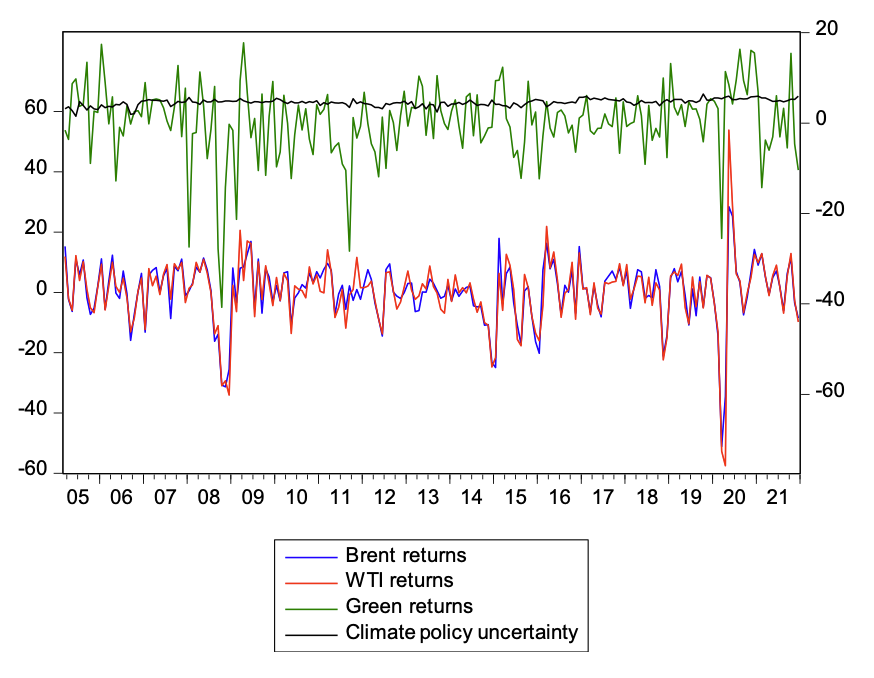
where $y_{r}$ is the return series and $\ y$ is the variable to be transformed into a return series. A careful observation of Figure 1 shows that Brent crude and WTI returns move in the same direction, with significant breaks identified and reported in Table 1.

Figure 1.Trends in Brent returns, WTI returns, green returns, and climate policy uncertainties

This figure shows the movements of Brent returns, WTI returns, green asset returns, and climate policy uncertainties from March 2005 to December 2021.

This figure shows the movements of Brent returns, WTI returns, green asset returns, and climate policy uncertainties from March 2005 to December 2021.

B. Methodology

We lay out the methodology adopted for the study in this section; this is the fractional differencing methodology. Traditional methods restrict integrated series to 0, 1, and 2. However, economic series can be fractionally integrated (Gil-Alana & Carcel, 2020). In fractionally integrated series, the impact of shocks is not assumed to be permanent, but transitory. We use the fractional integration approach to understand the time series properties of the series by estimating the following equation:

$$(1 - L)^{d}y_{t} = \alpha + \gamma Trend + \varepsilon_{t} \tag{2}$$

where $y_{t}$ is the vector of brent crude, WTI and green stock returns, and the log of climate policy uncertainty; $d$ is any real value; $L$ represents the lag operator such that $y_{t} = y_{t - 1}$; $(1 - L)^{d}$ is a polynomial function of order $d$; $\alpha$ is the model intercept; $\gamma$ is the trend coefficient; and $\varepsilon_{t} \sim N(0,\ \sigma_{\varepsilon}^{2})$. We can use the binomial expansion to reformulate the polynomial function, $(1 - L)^{d}$, in Equation (1) and thus:

$$\begin{align} (1 - L)^{d} &= \sum_{j = 0}^{\infty}{\tau_{j}L^{j}} = \sum_{j = 0}^{\infty}\begin{pmatrix} d \\ j \\ \end{pmatrix}( - 1)^{j}L^{j} \\ &= 1 - dL + \frac{d(d - 1)}{2}L^{2} - ..., \end{align} \tag{3}$$

$$\therefore$$

$$(1 - L)^{d}y_{t} = y_{t} - d\ y_{t - 1} + \frac{d(d - 1)}{2}y_{t - 2} - ..., \tag{4}$$

and Equation (2) becomes

$$\begin{align} y_{t} &= \alpha + \gamma Trend + d\ y_{t - 1} \\ &\quad - \frac{d(d - 1)}{2}y_{t - 2} - ... + \varepsilon_{t}. \end{align} \tag{5}$$

In Equation (5), $d$ is the degree of dependence of $y$. The higher the value of $d$, the more persistent the series is (Gil-Alana & Carcel, 2020). The parameter $d$ can fall into any of these three cases. We estimate d (and the corresponding 95% confidence intervals) considering: (i) the case of no deterministic trend, (ii) the model with an intercept, and (iii) the model with a linear time trend.

To confirm fractional cointegration on the multivariate series, we follow the two-step procedure of Gil-Alana et al. (2019) for the fractional case. This procedure is superior to the method of Johansen & Nielsen (2012), which imposes the same degree of integration on the system of equation.

We regress green asset returns on Brent crude returns and climate policy uncertainty. The equation is specified as:

$${GR}_{t} = \alpha + \sum_{i = 1}^{2}{\beta_{i}z_{it}} + x_{t},\ t = 1,2,\ldots, \tag{6}$$

where $z_{1t}$ is Brent crude return (BR) and $z_{2t}$ is climate policy uncertainty (CPU); $\beta_{0}$ is the intercept, $\beta_{1}$ is coefficient for Brent returns, and $\beta_{2}$ is coefficient for climate policy uncertainty. In the second step, we test the residual of Equation (6) for fractional integration. If the residual of the equation is fractionally integrated, we can conclude that there is fractional cointegration among the series.

We account for unknown structural breaks in each series followingthe three-step method of Salisu and Obiora (2021). First, we use the ADF method to determine the break dates in each series. Next, we construct a dummy variable for each of the break periods and we regress each of the variables on the dummy, illustrated in Equation (5)

$$y_{t} = \vartheta + \sum_{j = 1}^{N}{\iota_{j}D_{jt} + \mu_{t}} \tag{7}$$

where $y$ is the break-adjusted series; $D_{j}$is 1 for each $j$ and zero otherwise. Lastly, we determine the break-adjusted series by estimating $y_{t}^{d} = y_{t} - \sum_{j = 1}^{N}{{\widehat{\iota}}_{j}D_{jt}}.$ We test for persistence on the break-adjusted series.

To account for possible asymmetries in the return series, we decomposed Brent returns, WTI returns, green asset returns, and climate policy uncertainty into the positive and negative partial sums thus; $\sum_{j = 1}^{t}{\mathrm{\Delta}y_{j}^{+}} = \sum_{j = 1}^{t}{\max\left( \mathrm{\Delta}y_{j},0 \right)}$ and $\sum_{j = 1}^{t}{\mathrm{\Delta}y_{j}^{-}} = \sum_{j = 1}^{t}{min\ \left( \mathrm{\Delta}y_{j},0 \right)}$; where $y$ represents the four series to be decomposed.

III. Results

A. Is there persistence in Brent returns, WTI returns, green asset returns, and climate policy uncertainty?

In Table 1, the results show that there is significant short memory in Brent and WTI returns, given that the estimated d is statistically smaller than 1. There is no significance in fractional integration for the green asset returns. The implication is that the series as they are, except for green asset returns, have low persistence, and thus the shock effect does not last into the future. However, climate policy uncertainty shows high persistence but is mean reverting, given that the estimated d parameter is significantly greater than 0.

In the analysis of the partial sum of the series, we observe that Brent, WTI, and green asset returns are persistent but mean reverting, given that d > 0. The estimated d for the positive and negative partial sums of climate policy uncertainty is not statistically significant. Thus, climate policy uncertainty is not sensitive to shocks because of its positive and negative partial sums.

Furthermore, when the series are adjusted for structural breaks, it is observed that Brent and WTI returns exhibit short memory, as their estimated d parameter is significantly less than 1, while climate policy uncertainty exhibits long memory.

B. Are the series fractionally cointegrated?

Having established persistence (or fractional integration in some form), we test whether there is a long-run relationship between climate policy uncertainty, Brent returns, and green returns, using the positive and negative change in green asset returns as the dependent variables and green asset returns for the break-adjusted cointegration analysis. The results (in Table 2) show that there is no long-run fractional cointegration among the series.

Given the global reliance on fossil energy as the primary source of energy supply, when crises occur, it is unsurprising that the effect of climate policy uncertainty and Brent returns is not fractionally cointegrated with green returns, jeopardizing efforts to shift away from fossil to green energy.

C. Robustness Check

If we adopt WTI returns, will there still be no long cointegration? The results in Table 3 for the WTI returns are similar to those for Brent crude. There is no long-run fractional cointegration among the series.

IV. Conclusion

In this study, we used the fractional integration approach to study the persistence of Brent returns, WTI returns, green asset returns, and climate policy uncertainty. We find evidence of low persistence considering the series as are. The series, except for climate policy uncertainty, exhibit high persistence but are mean reverting when considering asymmetries. Except for green returns, Brent and WTI returns show low persistence after controlling for structural breaks, while climate uncertainty shows high persistence that is mean reverting. The study further shows that there is no long-term relationship among the persistent series.

This study is relevant to policymakers because it shows that policies on climate uncertainty must be such that they are more focused on long-term issues, since short-term measures may not last for long.