I. Introduction

Current events in the global arena, such as the emergence of the COVID-19 pandemic and the Russia-Ukraine War, have affected both the financial and energy sectors in different countries and have sparked renewed interest in the relationship between two market indicators—oil and stock returns.

The advent of the COVID-19 pandemic and the containment measures taken by governments across the world have caused significant disruptions to the global economy, especially the global financial and oil markets (Iyke & Ho, 2021; Raifu, 2022). Specifically, on April 21^st, 2020, West Texas Intermediate (WTI) oil price recorded a negative price of $36.98 per barrel, falling from $18.31 per barrel the previous day.^[1] Similarly, Brent crude oil price fell by 47.47% from $17.36 per barrel on April 20^th, 2020 to $9.12 per barrel on April 21^st, 2020.^[2] In the global financial market, Dow Jones, NASDAQ 100 and S&P 500 share prices declined on average by 0.56%, 0.27% and 0.53%, respectively, between March 11^th and March 31^st, 2020.^[3] Conversely, the current war between Russia and Ukraine has led to a significant spike in the prices of crude oil occasioned by crude oil supply disruption. Before the beginning of the war on February 24^th, 2022, WTI and Brent crude oil prices stood at $92.77 per barrel and $99.29 per barrel, respectively.^[4] Within a month, WTI and Brent crude oil prices rose significantly to $116.2 per barrel and $122.67 per barrel, respectively—a historical rise in oil returns since the Global Financial Crisis (GFC).^[5]

Theoretically, there is a negative relation between oil prices and stock returns through the cash flow channel (Jones & Kaul, 1996). However, the empirical evidence, in terms of impact and direction of causality, appears inconclusive (see Smyth & Narayan, 2018, for a review). Besides, global occurrences, such as the GFC, COVID-19 pandemic, and Russia-Ukraine War, do influence how oil prices affect different sectors of the economy. Such occurrences of global crises do cause a structural shift in the relationship between oil returns and stock returns, thereby affecting the directions of causality over time. Thus, failure to account for such structural changes when modelling the causality between oil returns and stock returns could lead to a spurious conclusion (Salisu & Fasanya, 2013).

In light of this, we hypothesize that there is no time-varying causality between oil returns and stock returns in Norway—the largest crude oil exporter in Europe (Singhal et al., 2021). To test this null hypothesis against the alternative, we use a time-varying causality method developed by Shi, Hurn, and Phillips (2018). This method has a couple of advantages. The most important of them is that it allows for changes in the causal directions, dating of economic crisis, and instability in the relationship between variables (Shi et al., 2018). Several studies have examined the causal relationship between oil returns and stock returns in Norway (see e.g., Bjørnland, 2009; Singhal et al., 2021), but none has examined the time-varying causal relation between oil returns and stock returns. In addition, this study examines the time-varying causality between oil returns and stock returns using daily, weekly, and monthly data of oil returns and stock returns.

The remaining sections are organised as follows: Section 2 presents the methodology and data sources. Section 3 presents findings, while Section 4 concludes.

II. Methodology and Data Sources

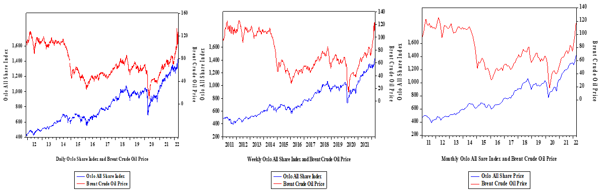
To model the time-varying causality between oil returns and stock returns in Norway, we use daily, weekly, and monthly data on Brent crude oil price and the OSLO All-Share index. The Brent crude oil price is obtained from the Energy Information Administration, while the OSLO All-Share index is sourced from https://www.investing.com. The data covers the period from 2011 to 2021. Figure 1 shows the trends of the daily, weekly, and monthly series of oil and stock prices. The returns to oil and stock are computed as follows:

$$\text{Oil returns:}\ \ln(\frac{olp}{olp_{t-1}})*100\tag{1}$$

$$\text{Stock returns:}\ \ln(\frac{stp}{stp_{t-1}})*100\tag{2}$$

The time-varying causality test developed by Shi et al. (2018) begins by specifying a lag-augmented VAR (LA-VAR) suggested by Toda and Yamamoto (1995). Assume a bivariate case of $x_{it}$ and $x_{2t},$ the LA-VAR model can be specified as:

$$\begin{aligned} &x_{i t}=\alpha_{10}+\alpha_{11 t}+\sum_{i=1}^{k+d} \beta_{1 i} x_{1 t-i}+\sum_{i=1}^{k+d} \delta_{1 i} x_{2 t-i}+\varepsilon_{1 t} \\ &x_{2 t}=\alpha_{20}+\alpha_{21 t}+\sum_{i=1}^{k+d} \beta_{2i} x_{2i1 t-i}+\sum_{i=1}^{k+d} \delta_{2 i} x_{2 t-i}+\varepsilon_{2 t} \end{aligned}\tag{3}$$

where $k$ is the lag length, $d$ is the maximum order of integration, and $t$ is the time trend. The null hypothesis of no Granger causality between $x_{1t}$ and $x_{2t}$ is specified as:

$$H_{0}: \delta_{11}=\cdot \cdot \cdot=\delta_{1 k}=0$$

The alternative hypothesis is specified as:

$$H_{0}: \delta_{11} \neq \cdot \cdot \cdot \neq \delta_{1 k} \neq 0$$

Given this LA-VAR framework, Shi et al. (2018) developed three supremum Wald tests that can be used to assess the time-varying causality between variables. These three supremum Wald tests include the forward recursive test of Thoma (1994), the rolling window test of Swanson (1998), and the recursive evolving algorithm test of Phillips, et al. (2015). Following Shi et al. (2018), the forward recursive algorithm Wald statistic $[f_1,f_2]$ with a small simple size fraction $f_w = f_2 - f_1 \ge f_0$ is given as $W_{f_{2}}(f_1)$ and the supremum Wald statistic version is given as:

$$s w_{F}\left(f_{0}\right)=\frac{\sup }{\left(f_{1}, f_{2} \in \wedge_{0}, f_{2}=f\right)}\left\{W_{f_{2}}\left(f_{1}\right)\right\} . \tag{4}$$

Here $\wedge_{0}=\left\{\left(f_{1}, f_{1}\right) ; 0 \prec f_{0}+f_{1} \leq 1\right.,$ and $\left.0 \leq f_{1} \leq 1-f_{0}\right\}$ for the small sample size $f_0 \in (0,1)$ in the regression. Shi et al. (2018) state that the forward expanding and rolling window are special cases of recursive evolving procedures, which have $f_1 = 0$ and sets $f = f_1.$ The rolling window itself has a fixed window width $f_w = f_2 = f_1 = f_0$ and window initialisation $f_1 = f_2 - f_1.$ The dating rules, especially in a simple switch case, are given for the three causality tests procedures as follows:

$$\begin{aligned} \text{Forward:}\ \hat{f}_{e} &=\frac{\inf }{f \in\left[f_{0}, 1\right]}\left\{f: W_{f}(0)>c v\right\}\\ \text{and}\ \hat{f}_{f} &=\frac{\inf }{f \in\left[f_{e}, 1\right]}\left\{f: W_{f}(0)>c v\right\} \end{aligned}\tag{5}$$

$$\begin{aligned} \text{Rolling:}\ \hat{f_{e}} &=\frac{\inf }{f \in\left[f_{0}, 1\right]}\left\{f: W_{f}\left(f-f_{0}\right)>c v\right\}\\ \text{and}\ \hat{f}_{f} &=\frac{\inf }{f \in\left[f_{e}, 1\right]}\left\{f: W_{f}\left(f-f_{0}\right)>c v\right\} \end{aligned}\tag{6}$$

$$\begin{aligned} \text{Recursive:}\ \hat{f}_{e} &=\frac{\inf }{f \in\left[f_{0}, 1\right]}\left\{f: S W_{f}\left(f_{0}\right)>s c v\right\}\\ \text{and}\ \hat{f}_{f} &=\frac{\inf }{f \in\left[f_{e}, 1\right]}\left\{f: S W_{f}\left(f_{0}\right)>s c v\right\} \end{aligned}\tag{7}$$

where $cv$ and $scv$ are critical values of $W_f$ and $SW_f$ statistics, respectively. The indicators $\hat{f_e}$ and $\hat{f_f}$ are estimated chronologically and their test statistics can exceed or fall below the critical values for the beginning and endpoints in the causal nexus.

Figure 1.Trends of the daily, weekly, and monthly oil and stock prices

III. Empirical Results

We conduct both the Augmented Dickey–Fuller and Phillips–Perron unit root tests. The results, presented in Table 1, show that the two oil and stock returns contain a unit root or are not stationary. Having determined the order of integration, we further conducted the structural stability test using the Quandt–Andrews and Bai–Perron structural breakpoint tests. The results from the two tests for all data frequencies are displayed in Table 2. The two tests support the evidence that oil and stock returns are unstable overtime, implying that there is a structural break in the data series, which occurred during the peaks of the COVID-19 pandemic (March and April 2020). For the daily, weekly, and monthly data, structural breaks occurred on 25^th March 2020, 15^th March 2020, and April 2020, respectively. This finding is in line with what was observed during the pandemic (Zhang et al., 2021).

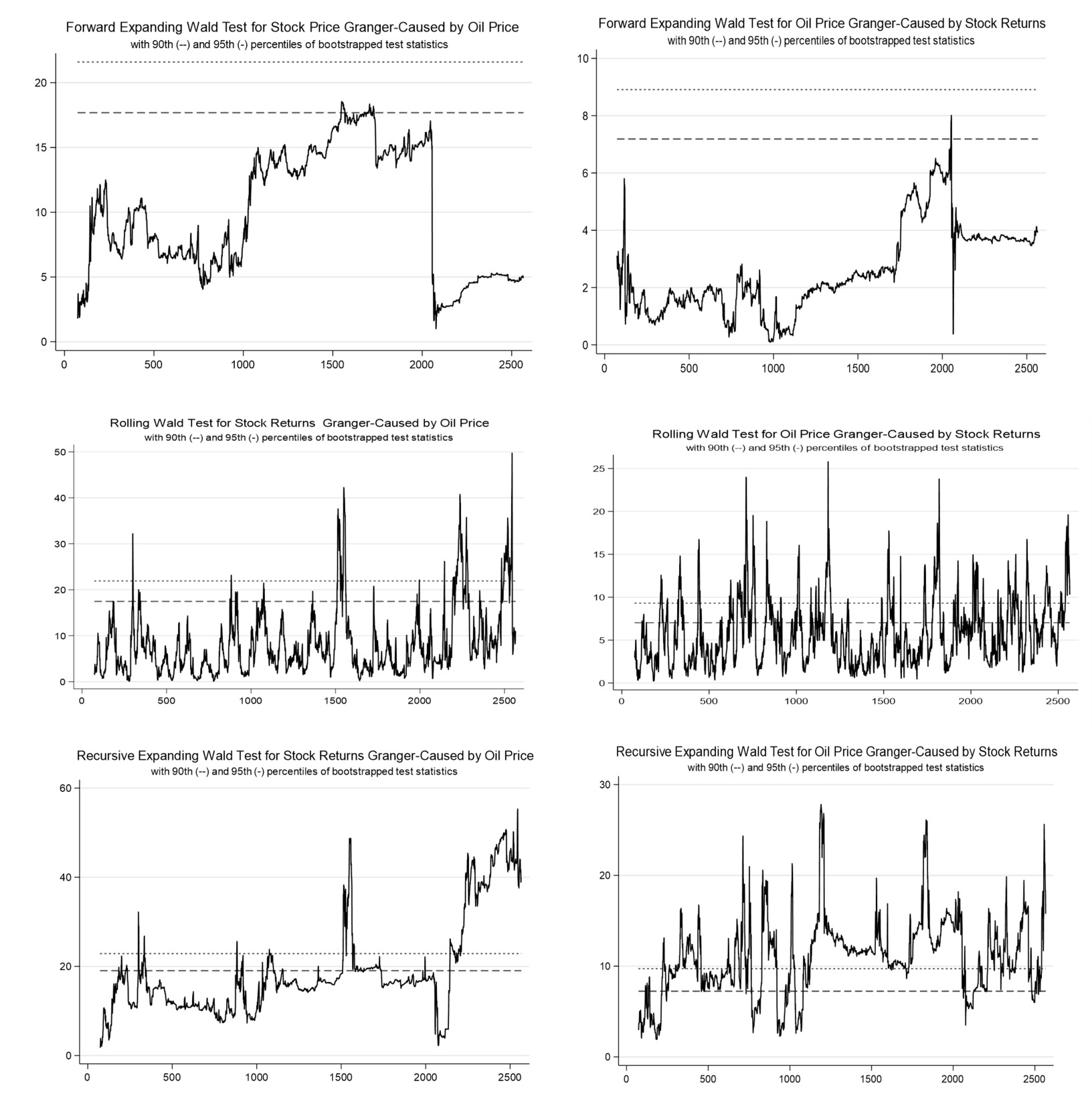
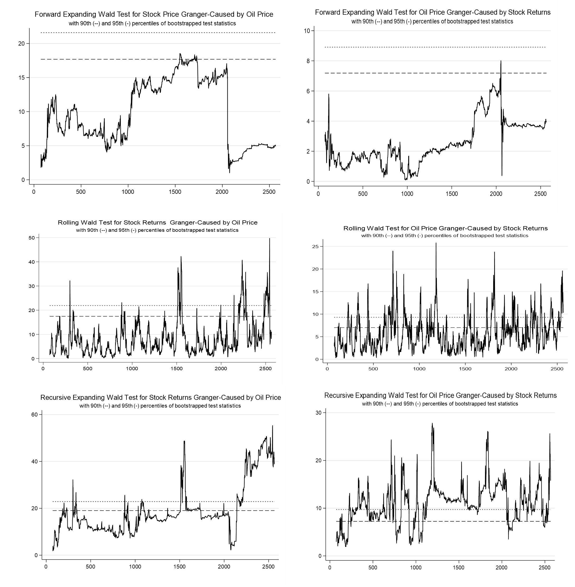
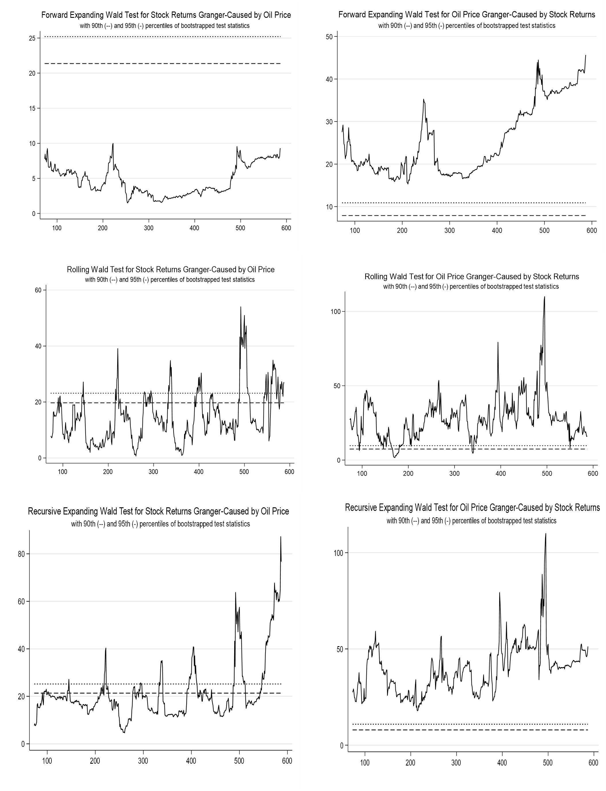
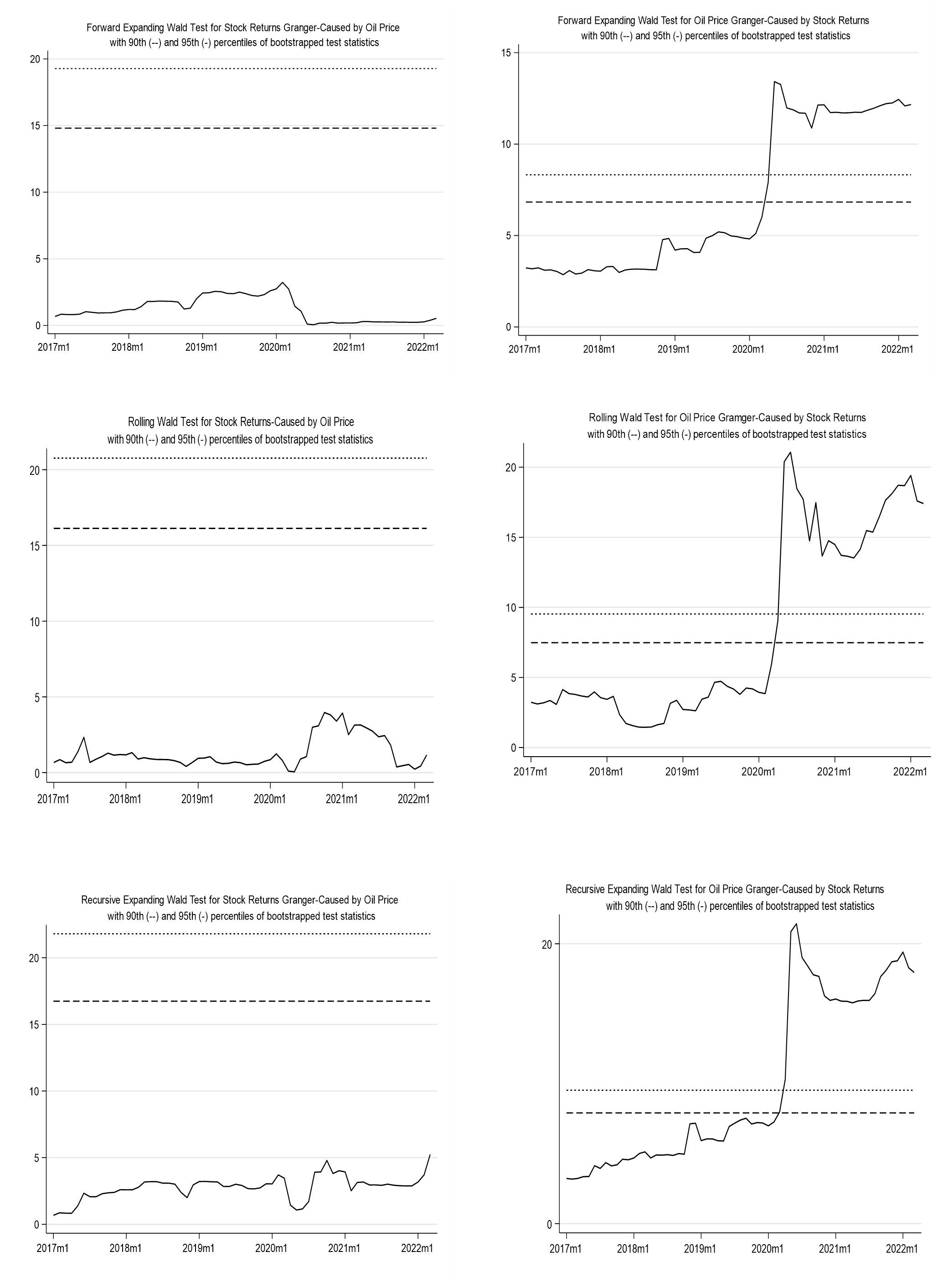
Table 3 presents the results of the linear and time-varying causality tests between oil returns and stock returns in Norway. For the linear causality, we use the Toda-Yamamoto Granger-non-causality test. The results for the weekly and monthly data show the existence of unidirectional causality running from stock returns to oil returns. However, the results from the daily data show that the causality runs from both sides—that is, from oil returns to stock returns and vice versa. When we apply the time-varying causality test, the results are a bit different for the daily and weekly data but are same for the monthly data irrespective of the algorithm procedures employed. Specifically, the results show that, though causality varies between oil returns and stock returns overtimes, the variability is dominated by unidirectional causality from stock returns to oil returns. This indicates that stock returns have predictive power over oil returns. This could be attributed to the fact that energy companies also trade in the stock market. Hence, whatever happens in the stock market, especially in the course of trading, could affect energy price. For weekly data, only the rolling algorithm procedure shows bidirectional causality between oil returns and stock returns. The recursive expanding algorithm procedure results show the existence of unidirectional causality that runs from oil returns to stock returns. However, the forward expanding algorithm procedure shows that there is no causality between oil returns and stock returns. For the daily data results, both the forward and rolling algorithm procedures support a bidirectional causality between oil returns and stock returns, while the recursive expanding algorithm procedure supports a unidirectional causality that runs from stock returns to oil returns (see Appendix for the time-varying causality graphs, which show the periods of causality).

IV. Conclusion

This study investigates the time-varying causality between oil returns and stock returns in Norway taking into consideration the data frequencies (daily, weekly, and monthly data). We find that data frequency determines the direction of causality between oil returns and stock returns. Specifically, we establish the existence of a bidirectional causality between oil returns and stock returns in daily data. In weekly and monthly data, we find the existence of a unidirectional causality that runs from stock returns to oil returns. Above all, we establish a time-varying causality between oil returns and stock returns, thereby rejecting the null hypothesis of no time-varying causality between the two variables. This study only assesses a time-varying causality between oil returns and stock returns in Norway. Future studies should include top global crude oil-exporting countries. We conclude that a strong policy is fundamental to building oil and stock markets’ resilience to the pandemic.

Acknowledgement

The author acknowledges insightful comments and suggestions from an anonymous reviewer and editor of this journal.