I. Introduction

In this paper, we investigate the day-of-the-week price persistence and seasonality in Spanish energy prices using an updated fractional persistence framework. We employ two recent nonlinear approaches, i.e., nonlinear I(d) frameworks recently proposed. The first is the Cuestas and Gil-Alana (2016) [CG2016] nonlinear I(d) method which is based on the Chebyshev polynomials in time, while the second is the Gil-Alana and Yaya (2021) [GY2021] method that relies on Fourier-form nonlinearity, a mimic of Enders and Lee (2012), in the fractional persistence framework. These two nonlinear functions allow for the smooth modelling of structural breaks in the time series. Bai and Perron’s (2003) multiple break test considers a maximum of five instantaneous breaks to be detected and in reality, breaks could be more than five in a given long time series, so, this test is restrictive, and in reality, some breaks are smoothly changing with time. Enders and Lee (2012) have found that a model with trigonometric function could have more power than the Bai-Perron break test in terms of modelling as many multiple breaks in a smooth fashion.

Fractional persistence allows for a given time series (i.e., energy price in this case) to be checked for the possibility of mean reversion or non-mean reversion. Another subset of the mean reversion case is long memory where a certain real value, $d,$ lies in the interval i.e., $0 < d < 0.5,$ where future values closely depend on the past lagged values since the autocorrelation function of the time series decay exponentially slowly, unlike the case of Autoregressive Moving Average (ARMA) process. Thus, this is the case of stationary mean reversion. Generally, mean reversion implies d lying in the range $0 < d < 1,$ including both stationary and nonstationary ranges. Thus, once the external shock triggers the time series process, there is the tendency for the series to revert to its mean level after a short time. The case of non-mean reversion is $(1 \leq d < 2),$ where it is unlikely for the series to revert to its mean level, even with strong government and regulator policies, and if at all, it will take a very long time. These are the appealing properties of the fractional persistence framework, which makes it distinguishable among classical unit root tests in the literature. Meanwhile, the Dickey-Fuller-like unit root test has been found to lack power in the presence of fractional unit root alternatives (Lee & Schmidt, 1996).

Energy pricing and its distribution, as it affects households and businesses, is one of the major global discussions. The present work is motivated by the alarmingly rising electricity prices in Spain since July 2021 due to the global gas crisis. Findings here will therefore guide regulators and the government on the price dynamics of electricity in Spain.

II. Nonlinear Fractional I(d) frameworks

Following Granger and Joyeux (1980) and Hosking (1981), we define fractional integration in time series as,

$$(1 - L)^d x_t = \tilde{\varepsilon}_t \tag{1}$$

where $L$ is the lag operator, i.e., $L^q y_t = y_{t-q},$ $d$ is the fractional integration parameter operating on the differencing operator $(1 - L)^d$ on the time series $y_t$ to produce a stable/stationary series $\varepsilon_t$ that has the properties of white noise. In some cases of highly autocorrelated series, we can consider the possibility of Autoregressive [AR(1)] error disturbance, i.e.

$$\tilde{\varepsilon} = \theta_1 \tilde{\varepsilon}_{t-1} + v_t \tag{2}$$

where $\theta_1$ is the AR(1) parameter for $\tilde{\varepsilon}_{t-1}$ which is the first lag of $\tilde{\varepsilon}_{t},$ and $v_t$ is some noise process. Much recently, the applicability of the operator d (1) has gone beyond unit root testing of time series to testing persistence of series in terms of mean or non-mean reversions. By extending the above to using the deterministic term of a linear trend with constant, $\alpha$ and intercept, $\beta ,$ one obtains the Robinson (1994) fractional persistence modelling framework,

$$y_t = \alpha + \beta t + x_t,\quad (1 - L)^d x_t = \tilde{\varepsilon}_t, \quad t = 1, 2, \dots , \tag{3}$$

which is estimated using the Ordinary Least Square (OLS) estimation method, i.e,

$$\tilde{\varepsilon}_t = y^*_t - \hat{\alpha}_0 1^*_t + \hat{\beta}t^*_t, \tag{4}$$

and $y^*_t = (1-L)^{d_o}y_t: 1^*_t = (1-L)^{d_o} 1_t: t^*_t = (1-L)^{d_o} t_t,$ with the complex Lagrange Multiplier test statistic,

$$\hat{R} = \frac{T}{\hat{\sigma}^4} \hat{a^1} \hat{A}^{-1} \hat{a},\tag{5}$$

where $T$ is the sample size, and

$$\begin{aligned} \hat{\mathrm{a}}&=\frac{-2 \pi}{\mathrm{T}} \sum_{\mathrm{j}}^{*} \psi\left(\lambda_{\mathrm{j}}\right) g_{\mathrm{u}}\left(\lambda_{\mathrm{j}} ; \hat{\tau}\right)^{-1} \mathrm{I}\left(\lambda_{\mathrm{j}}\right) ; \\ \hat{\sigma}^{2}&=\sigma^{2}(\hat{\tau})=\frac{2 \pi^{\mathrm{T}}-1}{\mathrm{~T}} \sum_{\mathrm{j}=1} \mathrm{~g}_{\mathrm{u}}\left(\lambda_{\mathrm{j}} ; \hat{\tau}\right)^{-1} \mathrm{I}\left(\lambda_{\mathrm{j}}\right), \\ \hat{A}&=\frac{2}{T}\bigg\{\sum_{j}^{*} \psi\left(\lambda_{j}\right) \psi\left(\lambda_{j}\right)^{\prime} \\ &\quad - \sum_{j}^{*} \psi\left(\lambda_{j}\right) \hat{\xi}\left(\lambda_{j}\right)^{\prime}\left[\sum_{j}^{*} \hat{\xi}\left(\lambda_{j}\right) \hat{\xi}\left(\lambda_{j}\right)^{\prime}\right]^{-1}\\ &\quad \times \sum_{j}^{*} \hat{\xi}\left(\lambda_{j}\right) \psi\left(\lambda_{j}\right)^{\prime}\bigg\} ; \\ \psi\left(\lambda_{j}\right)&=\log \left|2 \sin \frac{\lambda_{j}}{2}\right| ; \\ \hat{\xi}\left(\lambda_{j}\right)&=\frac{\partial}{\partial \tau} \log g_{\varepsilon}\left(\lambda_{j} ; \hat{\tau}\right),\\ \lambda_{\mathrm{j}}&=2 \pi \mathrm{j} / \mathrm{T}, \end{aligned}$$

and $*$ implies that the sums are taken over all frequencies that are bounded in the spectrum, with periodogram $\text{I}(\lambda_\text{j})$ for $\tilde{\varepsilon}_t$ and $\hat{\tau} = \arg \min_{\tau \varepsilon T^*}\sigma^2(\tau)$.

The linear I(d) framework of Robinson (1994) is extended to the nonlinear I(d) framework in Cuestas and Gil-Alana (2016) by using the function $f(t)$ which depends on unknown parameters $\theta_i\ (i = 1,2,\dots,m)$ in the I(d) framework,

$$\begin{aligned} (1-L)^{d} y_{t} &=\alpha+f(t)+\tilde{\varepsilon}_{t} \\ & \cong \theta_{0}+\sum_{i=1}^{m} \theta_{i} \mathrm{P}_{i, T}(t)+\tilde{\varepsilon}_{t},\\ t &= 1,2, \ldots, i=1, \ldots, m \end{aligned}\tag{6}$$

where $\theta_0$ is the constant and $\theta_i$ are the parameters of the m^th order expansion of the Chebyshev polynomial

$$\begin{aligned} \text{P}_{i,t}(t) &= \sqrt{2}\cos[i \pi (t - 0.5)/T],\\ t &= 1,2,\dots,i = 1,\dots,m \end{aligned}\tag{7}$$

and $\pi = 3.142.$ Then, in the absence of nonlinearity, the I(d) model in (6) is expressed with only a constant, if $m = 1,$ the model becomes a linear I(d) model of Robinson (1994) with a linear trend. For $m > 1,$ the model becomes nonlinear such that the higher the order of $m,$ the higher the nonlinearity. We can re-express the model in (7) for a truncation order of $m = 3$. For simplicity of OLS estimation, (y7) in Equation (6) is expressed as,

$$\tilde{\varepsilon}_t = y^*_t - \alpha 1^*_t - \cos 1^* - \cos 2^* - \cos 3^* \tag{8}$$

where

$$\begin{gathered} y_{t}^{*}=(1-L)^{d_{a}} y_{t},\\ 1_{t}^{*}=(1-L)^{d_{d}} 1_{t},\\ \cos 1^{*}=(1-L)^{d_{n}} \sqrt{2} \cos [\pi(t-0.5) / T],\\ \cos 2^{*}=(1-L)^{d_{n}} \sqrt{2} \cos [2 \pi(t-0.5) / T]\\ \text{and}\\ \cos 3^{*}=(1-L)^{d_{0}} \sqrt{2} \cos [3 \pi(t-0.5) / T]. \end{gathered}$$

As a follow-up to Cuestas and Gil-Alana’s (2016) method, Gil-Alana and Yaya (2021) considered using flexible Fourier fractional (FFF) form

$$f(t)=\sum_{k}^{n} \lambda_{k} \sin \left(2 \pi j_{k} t / T\right)+\sum_{k}^{n} \gamma_{k} \cos \left(2 \pi j_{k} t / T\right)$$

in the I(d) structure in Equation (6) to mimic the nonlinearity induced by function $f(t),$ where $n$ is the optimal FFF value, $n = j_k;$ $k$ a particular frequency which could be fractional or unit; $\lambda_k$ and $\gamma_k$ determine the amplitude and displacement of the sine/cosine in the Fourier function. Thus, the nonlinear I(d) is,

$$\begin{aligned} (1-L)^{d} y_{t} &= \alpha \\ &\quad +\bigg\{\sum_{k}^{n} \lambda_{k} \sin \left(2 \pi j_{k} t / T\right)\\ &\quad +\sum_{k}^{n} \gamma_{k} \cos \left(2 \pi j_{k} t / T\right)\bigg\}\\ &\quad +\tilde{\varepsilon}_{t} \end{aligned} \tag{9}$$

Empirically, (9) can be re-expressed as,

$$\tilde{\varepsilon}_{t} = y_{t}^{*}-\alpha 1_{t}^{*}-\sum_{k}^{n} \lambda_{k} \sin _{k, t}^{*}-\sum_{k}^{n} \gamma_{k} \cos _{k, t}^{*}, \tag{10}$$

where

$$\begin{gathered}\sin _{k, t}^{*}=(1-L)^{d_{0}} \sin \left(2 \pi j_{k} t / T\right),\\ \cos _{k, t}^{*}=(1-L)^{d_{0}} \cos \left(2 \pi j_{k} t / T\right)\end{gathered}$$

with $y^*_t$ and $1^*_t$ defined in (7) above.

III. Data and Results

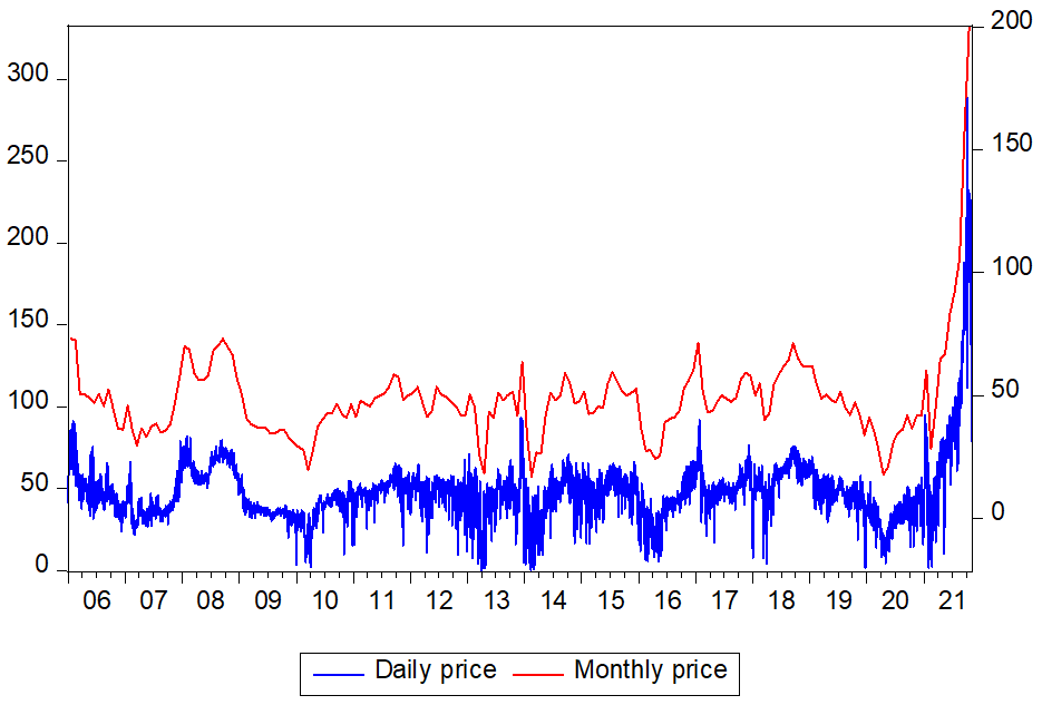
Daily historical spot prices of electricity for Spain, spanning 01/01/2006 to 04/11/2021, covering a total of 5788 data points, are obtained from the website of Iberian Energy Market Operator/Operador del Mercado Ibérico de la Energía-Polo Portugués (OMIP) at https://www.omip.pt/en/electricity. Plots of daily and monthly electricity prices are given in Figure 1. For daily prices, there are fluctuations over time and occasional price swings that are pronounced to both up and down prices. Between 2006 and June 2021, prices hover between 50 and 150 euro/MWh while prices started increasing astronomically in the middle of 2021.^[1] The average monthly pricing is superimposed on the daily price, and the essence of this is to check for possible monthly seasonal movement. By looking at the plot, the monthly seasonality is not observed.

Figure 1.Plot of electricity prices in Spain based on daily energy auctions

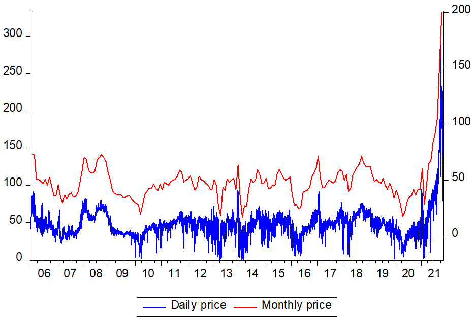
Table 1 presents the results of persistence using nonlinear smooth trend functions by employing the Chebyshev polynomial in time and Fourier function. In the case of the Chebyshev polynomial, the nonlinear trigonometric parameters, cos1, cos2 and cos3 are not significant, while in the case of Fourier function, the trigonometric parameter sin_k is only significant with the optimal Fourier frequency k = 0.46. For both the Chebyshev polynomial and Fourier function, fractional persistence values are 0.6739 and 0.6702 respectively under white noise disturbance and each estimate with an upper CI bound of about 0.69. To check for the possible interference of unchecked serial correlations in the model residuals which could bias our results, we allow for an AR(1) error disturbance instead of the white noise error disturbance, with the specification given in Equation (2). The results for both nonlinear I(d) are then re-presented in the lower panel of Table 1. In this case, cos2 parameter in the Chebyshev function is found to be significant, while sin_k parameter in the Fourier function is also significant. For both nonlinear functions, the AR(1) parameter estimates are low, around 0.20, but this is significant at 5% level. The persistence values estimated for both nonlinear I(d) models are found to be lower compared to the corresponding values under the white noise error disturbances. These values are found to be 0.5601 and 0.5548 respectively, which is around 0.5 implying mean reversion with long-range dependence characteristics in the electricity prices.

The analysis is extended by obtaining the day-of-the-week series persistence using the two nonlinear I(d) frameworks and the results, as presented in Table 2, are only reported for the case of AR(1) error disturbance. In the upper panel of the results table for the case of Chebyshev polynomial I(d), it is found that none of the nonlinear parameters for the days-of-the-week series (i.e., Monday–Friday) is significant while for Wednesday, Saturday and Sunday series, nonlinear parameters are significant. The AR(1) parameters are significant for Wednesday, Saturday and Sunday series. The persistence estimates for the seven series are 0.65 (Monday), 0.73 (Tuesday), 0.78 (Wednesday), 0.77 (Friday), -0.30 (Saturday) and -0.39 (Sunday). By looking at the results in the lower panel of the table for the Fourier function, with optimal Fourier frequency k recorded in the last column of the table, the significance of Fourier form parameters (sine and cosine) are observed. Thus, the results in Table 2 confirm the nonlinear nature of day-of-the-week in Spanish electricity prices. The persistence results, though, all in mean reverting ranges, are in the interval 0.62–0.77. The persistence on Monday, Saturday and Sunday are 0.64, 0.69 and 0.64 respectively while others (Tuesday–Friday) are in the range of 0.71–0.77.

To probe further for possible monthly seasonality, the monthly dataset is estimated by employing a seasonal AR model in the nonlinear I(d) frameworks. Thus, we re-specify (2) as

$$\tilde{\varepsilon} = \theta_{12} \tilde{\varepsilon}_{t-12} + v_t\tag{11}$$

where $\theta_{12}$ is the seasonal AR parameter in the case of monthly time series, and $\tilde{\varepsilon}_{t-12}$ is the lag 12 of the resulting fractionally differenced series. Thus, $\theta_{12}$ determines the monthly seasonal autoregression between the previous 12th observation (i.e., $\tilde{\varepsilon}_{t-12})$ and the current observation, $\tilde{\varepsilon}_t.$ The model in Equation (11) is then analyzed with Equations (8) and (10) to obtain results for the Chebyshev polynomial and Fourier function respectively. The results of the Chebyshev polynomial reported in the upper panel of the results table indicated non-significance of seasonal AR parameter with a very low coefficient (0.0816). Meanwhile, the fractional persistence estimate is computed as 0.9323 which is quite higher than that obtained for the case of daily pricing. Similar results are obtained in the case of the Fourier function presented in the last panel of Table 3, where the non-significance of the seasonal AR parameter with nonlinearity detected as $\cos_k$ is found to be significant at the 5% level.

IV. Concluding remarks

Energy pricing and its distribution are some of the major global discussions because they affect households and businesses. This study is motivated by the alarmingly rising electricity prices in Spain since July 2021 due to the global gas crisis. Thus, the findings in this study guide regulators and the government to know the price dynamics of electricity in Spain. We employed updated fractional persistence frameworks in nonlinear settings in investigating how day-of-the-week affects persistence and seasonality in the pricing from 01/01/2006 to 04/11/2021. Results obtained indicate mean reversion in prices across all days of the week and there is a fair increase in persistence during the working days (Tuesday, Wednesday, Thursday and Friday) compared to weekend days. No evidence of seasonality is found in the monthly price series. It is hoped that the results obtained here will guide in making energy usage policies in Spain.

Acknowledgements

Comments of the Editor and reviewers are gratefully acknowledged.