GMM Approach to Residential Electricity Consumption in Indonesia

I. Introduction

A key goal of the Indonesian government is to reach 100% national electrification ratio (Asian Development Bank, 2021). While this goal is nearly reached, with a figure of 92.95% for the overall sample of Indonesia in 2020 according to PT Perusahaan Listrik Negara (PLN)^[1] Annual Reports, cases of electricity poverty in some provinces, such as Papua, Nusa Tenggara Timur, and Sulawesi Barat, remain. The government seeks to provide electricity accessibility for most of society, particularly for households (Burke & Kurniawati, 2018). The issue of what drives electricity consumption among households cannot, therefore, be overestimated.

Examining households’ consumption of electricity in Indonesia is crucial for economic growth and the development of living standards, as well as for energy policy. First, Indonesia has a population of 273.52 million and is currently experiencing rapid urbanization. The total residential electricity demand rose from 84.1 TWh in 2014 to 111.4 TWh in 2020, amid an annual population growth of 0.98% (Indonesian Statistics, 2021). Demand for electricity is expected to grow even further. Second, Indonesia wants to ensure universal access to electricity, in line with Sustainable Development Goal 7. Currently, during the COVID-19 recovery situation, Indonesia is focusing on investment in social protection, such as increasing the number of households with access to PLN electricity (PT PLN, 2021).

Previous studies have revealed mixed results on the influence of income and price on electricity consumption (Arnaz, 2018; Fatmawati, 2021; Kusumaningrum, 2018). This suggests the need to reinvestigate the socioeconomic factors that could have led to changes in household demand for electricity from 2014 to 2020. The study contributes to the literature by applying generalized method of moments (GMM) estimation in two dynamic panel models.

II. Empirical Review

A wide array of studies has looked into the various factors affecting the demand for electricity. These studies can be classified as covering: 1) the causal relation between income and price (Arnaz, 2018); 2) the relations between income, prices, and demographic factors (population, urbanization, the Human Development Index, etc.; see Azam et al., 2015; Fatmawati, 2021); and 3) the linkage between income, prices, and government subsidies (Burke & Kurniawati, 2018; Safiah et al., 2021; Supriadi et al., 2019). Researchers have focused on investigating electricity prices and household income as the major determinants of residential energy consumption. From a macroeconomic perspective, studies (Azam et al., 2015; Fatmawati, 2021; Hartono et al., 2020) employing different methodologies have identified the gross domestic product per capita as having a positive and significant effect on households’ electricity demand. From a microeconomic perspective, Kusumaningrum (2018) investigated two household groups, with low and high volt–ampere installed power, respectively. Using quantile regression, the author found that, although both groups have income-inelastic demand for electricity, the latter is more responsive to income changes. Arnaz (2018), employing system GMM, found that income levels drive electricity consumption in Java–Bali and non-Java–Bali regions. Meanwhile, both Arnaz (2018) and Kusumaningrum (2018) showed that price changes affect residential electricity consumption.

The views on subsidy reforms that aim at providing universal access to electricity are also mixed. Burke and Kurniawati (2018) found that subsidy reductions induced savings in annual electricity usage relative to the no-reform counterfactual. However, the partial removal of subsidies, thus raising effective tariffs, led to the diminished welfare of households (Supriadi et al., 2019). Moreover, employing the autoregressive distributed lag method, Safiah et al. (2021) showed long-term cointegration between electricity consumption and economic growth. Energy subsidies, albeit aimed at short-term economic growth, have a nonsignificant influence on electricity consumption. Additionally, there were empirical observations that energy subsidies do not reach the target beneficiaries (Kusumaningrum, 2018).

While the foregoing researchers agreed that electricity prices and household incomes (including consumption across rural–urban areas and different income levels) remain the major determinants of energy consumption, mixed empirical results still abound, owing to differences in the nature of the data, periods, and research methodologies.

III. Data and Econometric Approach

A. Data

Our dataset covers 33 provinces of Indonesia (Kalimantan Timur and Kalimantan Utara combined) from 2014 to 2020. These provinces are located on six major islands, namely, Sumatera, Java, Bali and Nusa Tenggara, Kalimantan, Sulawesi, and Maluku and Papua. Annual data were collected from various sources. These include data on residential electricity consumption (GWh), average electricity tariffs, numbers of households, and the electrification ratio, obtained from the PT PLN Annual Reports, as well as the gross regional domestic product (GRDP) per capita in terms of thousands of constant 2010 rupiah prices, the population size, and the mean number of years of schooling, obtained from the Central Bureau of Statistics (Badan Pusat Statistik). Table 1 presents the descriptive statistics of the households across provinces from 2014 to 2020.

Total electricity consumption across the provinces increased each year, rising by 34.16% from 2014 to 2020, which can be attributed to the expanded electrification (by 19.8 percentage points) and the population growth. Interestingly, electricity consumption per household continued to decline over the years, but recovered slightly in 2020. This result could be linked to the general increase in electricity tariffs, albeit displaying fluctuations throughout the seven-year period. The average GRDP per capita underwent an annual growth of 3–4% from 2014 to 2019, but contracted by 3% in the following year. It is worth noting that the income per capita differential between provinces reached as high Rp 28.17 million (or USD 1,962). Meantime, household size and the mean of the number of schooling years remained stable.

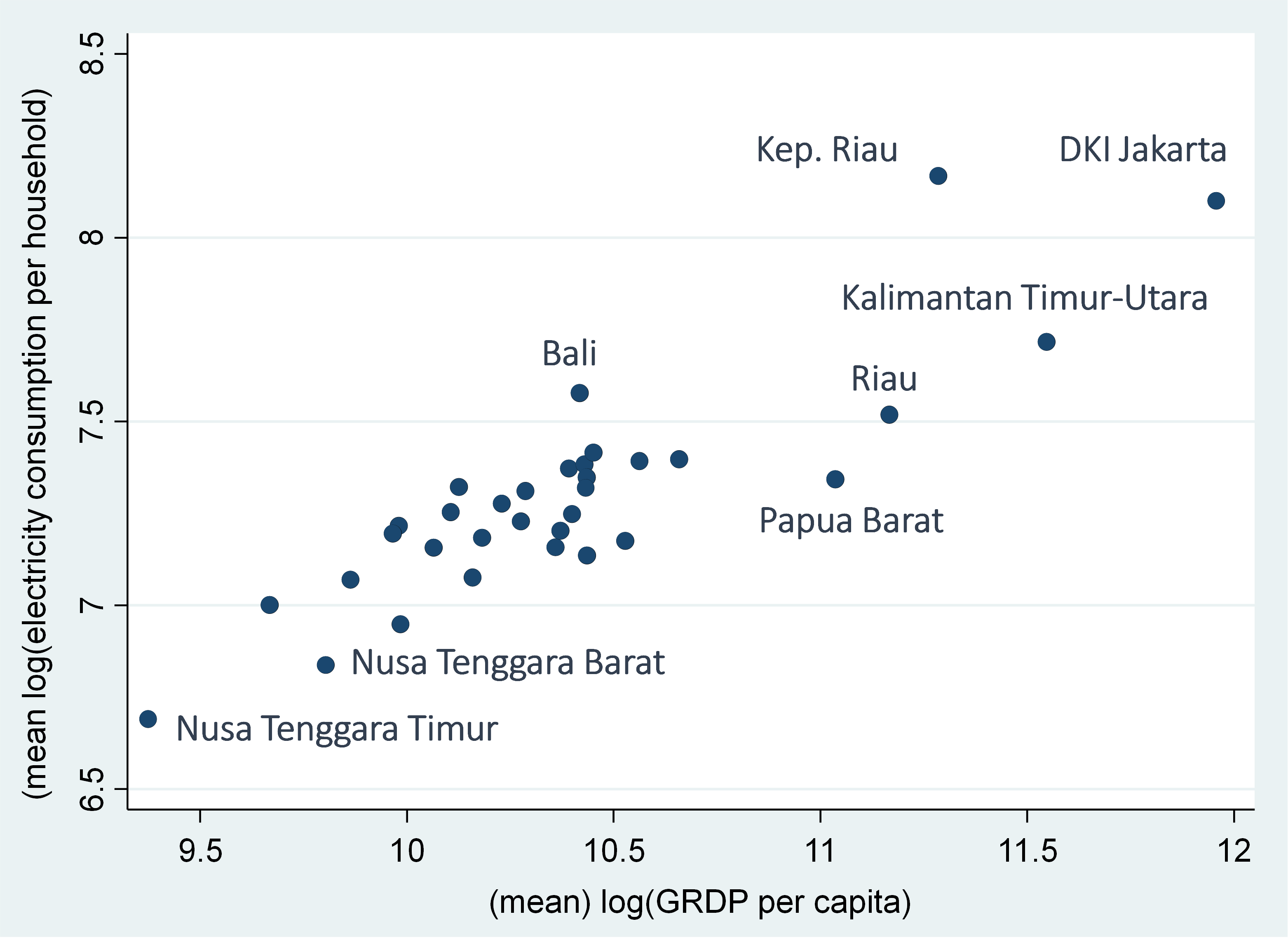
Figures 1 and 2 provide information on the provincial mean electricity consumption across GRDP per capita levels and tariff rates from 2014 to 2020. Kepulauan Riau and Daerah Khusus Ibukota Jakarta recorded the highest average electricity consumption per household throughout the seven-year period, whereas Nusa Tenggara Barat and Nusa Tenggara Timur had the lowest. A wide gap is also apparent in terms of economic size across provinces. The wealthiest provinces tend to have higher demand for electricity per household than their poorer counterparts.

Figure 1.Provincial mean electricity consumption across GPD per capita in logarithm (2014-2020).

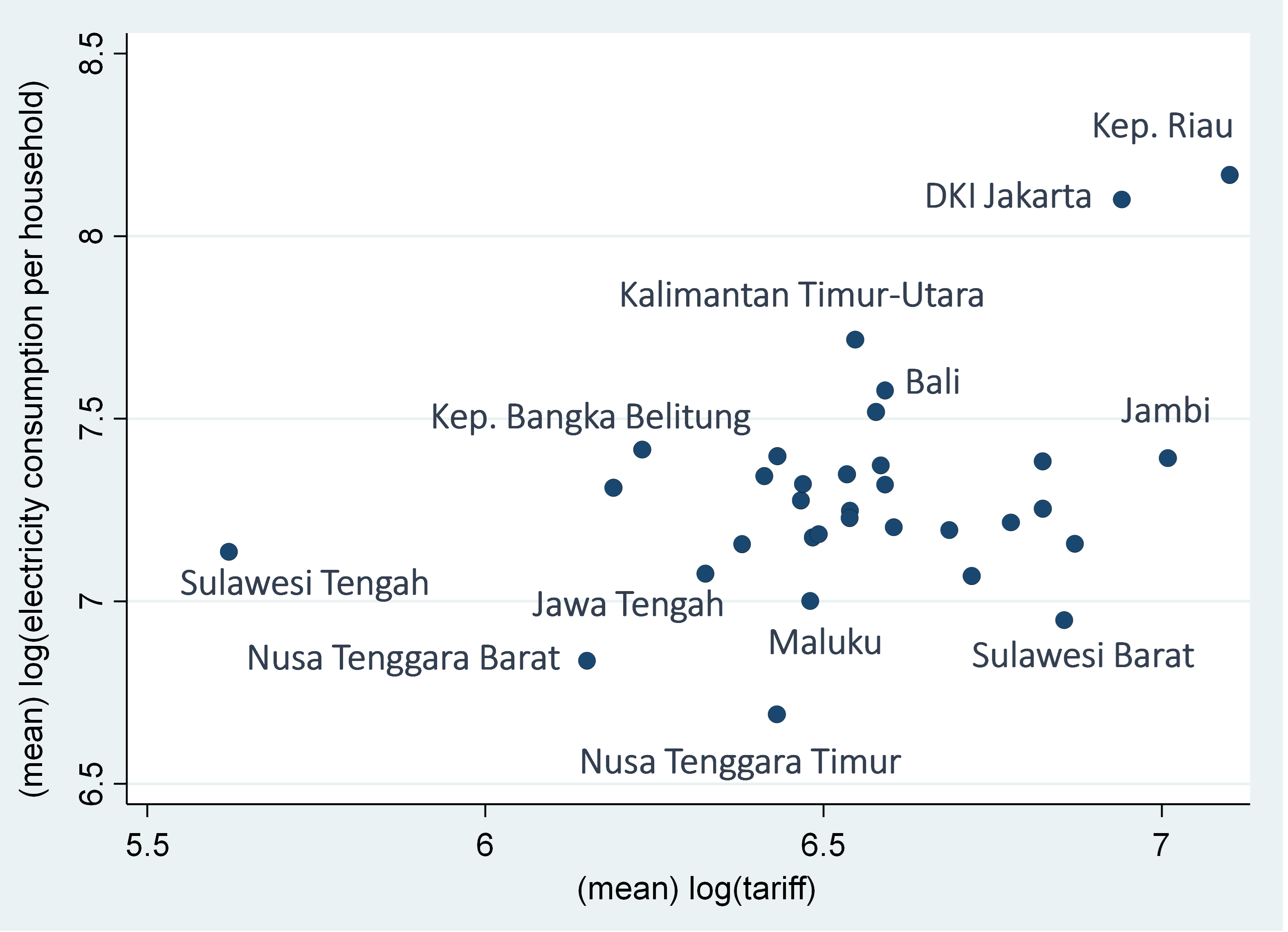
As aforementioned, average tariff rates have exhibited an erratic trend and, in 2020, dropped to Rp 1,016.50/KWh. Electricity prices in Indonesia are set by the government and based on group tariff structures, where a higher marginal per-KWh tariff is paid at higher usage levels. Nonetheless, no apparent trend can be discerned between electricity consumption per household and tariff rates (Figure 2). Around 18 provinces continued to be charged tariffs above the national level.

Figure 2.Provincial mean consumption across tariff rates in logarithm (2014-2020).

B. Econometric Approach

We employ two dynamic panel data models to investigate the factors affecting the demand for electricity. The first model uses the electricity consumption per household as the dependent variable, while the second model uses the aggregate electricity consumption of the residential sector. We specify a dynamic log-linear equation in which the electricity consumption and all the regressors, except the electrification ratio, are in natural logarithms, as follows, and the coefficients are thus interpreted as demand elasticities:

$$\begin{align} \log\left(Ch_{t}^{i} \right) &= \beta_{0} + \ \beta_{1}\log\left(Ch_{t - 1}^{i} \right) + \ \beta_{2}\log\left( Y_{t}^{i} \right)\\ &+ \ \beta_{3}\log\left( P_{t}^{i} \right)\ + \ \beta_{4}\log\left(HS_{t}^{i} \right)\\ &+ \ \beta_{5}\log\left( EDU_{t}^{i} \right) + \ \beta_{6}ER_{t}^{i}\\ &+ \ \sum_{y = 1}^{7}{\delta^{y}D_{t}^{y}}\ + \ u_{t}^{i} \end{align}\tag{1}$$

where $Ch_{t}^{i}$ is the electricity consumption per household in province $i$ in year $t,$ $Ch_{t - 1}^{i}$ is the electricity residential consumption per household in period $t - 1,$ $Y_{t}^{i}$ is the GRDP per capita in terms of thousands of constant 2010 rupiah prices, $P_{t}^{i}$ is the electricity tariff, $HS_{t}^{i}$ is the household size, $EDU_{t}^{i}$ is the mean of the number of schooling years, and $ER_{t}^{i}$ is the electrification ratio. The $D_{t}^{y}$ terms are seven-year dummies treated as strictly exogenous and uncorrelated with province-specific effects and are hence instrumented by themselves (Kripfganz, 2019; Roodman, 2009). The term $u_{t}^{i}$ is the error component, and it contains province-specific fixed effects and the regular disturbance term, assumed to be independent and identically distributed.

The second model has essentially the same independent variables as in the first model, except for $HS_{t}^{i},$ which is replaced by $POP_{t}^{i},$ referring to the total provincial population:

$$\begin{align} \log\left(Ch_{t}^{i} \right) &= \beta_{0} + \ \beta_{1}\log\left(Ch_{t - 1}^{i} \right) + \ \beta_{2}\log\left( Y_{t}^{i} \right)\\ &+ \ \beta_{3}\log\left( P_{t}^{i} \right) + \ \beta_{4}\log\left(POP_{t}^{i} \right)\\ &+ \ \beta_{5}\log\left(EDU_{t}^{i} \right) + \ \beta_{6}ER_{t}^{i}\\ &+ \ \sum_{y = 1}^{7}{\delta^{y} \cdot \ D_{t}^{y}}\ + \ u_{t}^{i} \end{align}\tag{2}$$

A dynamic panel model is utilized, since the time periods (T = 7) are smaller than the cross section of provinces (N = 33), where all the asymptotic properties of the GMM estimator rely on the size of the cross-sectional dimension of the panel. Dynamic panel regression is characterized by two sources of persistence, namely, autocorrelation and heterogeneity arising from unobserved individual-specific effects (Baltagi, 2021). The GMM estimator is preferred because it eliminates province-specific effects and any time-invariant province-specific variables (Arellano & Bond, 1991). In particular, we use the system GMM Blundell–Bond estimator, which combines the level and difference equations by using the lagged first differences of the regressors as instruments for the level equation, to eliminate simultaneity bias (Blundell & Bond, 1998). A two-step GMM estimator with robust standard errors is used, because the proliferation of instruments can lead to biased standard errors and parameter estimates. The first step ensures that the error terms are both independent and homoscedastic across provinces and over time, that is, there is no autocorrelation, while the second step tests for second-order serial correlation.

IV. Estimation Results and Discussion

The choice of dynamic panel models is justified because of the significance of the lagged value of electricity consumption in both model specifications (Table 2). Post-estimation tests, such as the Sargan test, reveal valid overidentification restrictions, implying the exogeneity of instruments. We find no second-order serial correlation for the disturbances of the first-differenced equation.

The sign of the lagged dependent variable varies between the two models. Arnaz (2018) showed that the previous value of electricity consumption per household affects future consumption. However, plotting the electricity consumption per household by province over time produces a somewhat flat line. We find no evidence that tariffs influence the demand for electricity in either model, although the negative sign of the coefficient is in accordance with theory. This result begs the question of the continuous electricity relief schemes implemented by the government despite previous subsidy reforms. The GRDP per capita is positive and significant in both models, suggesting that higher income induces electricity consumption, as expected. A percentage change in income is associated with a 0.58% increase in household electricity demand in the short run, exhibiting income inelasticity. In the long run, the income effect is smaller at 0.45% but still strongly significant. At the household level, education seems to matter, although the sign is counterintuitive. More educated households are expected to know how to conserve electricity, yet are more likely to use electricity-powered gadgets. At the aggregate level, the population size and electrification ratio affect electricity demand, with both long-run effects outweighing the short-run effects. In terms of time effects, only the years 2015 to 2017 under the first model are significant.

V. Conclusion

Following Sustainable Development Goal 7, this study focuses on residential electricity consumption during 2014–2020 in Indonesia by employing a system GMM estimator for two dynamic panel models. We find evidence that the GRDP per capita has a significant positive impact on the electricity demand per household. Moreover, the population size and electrification ratio affect the aggregate demand for electricity, suggesting that the ongoing government policies of improving access to electricity are effective. Tariffs as a proxy for price are not significant, however. For future research, the inclusion of more household characteristics in the model is important to investigate the poverty and distributional impact of any policy shifts on household consumption behavior during the pandemic.