I. INTRODUCTION

Behavioral finance theory posits that economic agents’ sentiments about the future economic developments may drive the economy because they influence agents’ decisions today—a view that may reflect rational arguments and facts but also a mood of optimism or pessimism (Nowzohour & Stracca, 2020), which plays a pivotal role in explaining economic activities and commodity prices. Moreover, according to noise trader theory that is mainly based on investor sentiment, investors’ trade behavior is subject to their bullish or bearish sentiment (Solanki & Seetharam, 2018).

The literature has extensively studied the impact of investor sentiment on economic activities (Baker & Wurgler, 2007; Dergiades, 2012; Zi-Long et al., 2021). Investor sentiment affects not only economic activities, but also oil prices. Indeed, the investor sentiment–oil price nexus has a prominent place in the behavioral finance literature. Besides macroeconomic variables, according to Qadan and Nama (2018), He et al. (2019), and Perifanis and Dagoumas (2021), behavioral elements such as investor sentiment also play a significant role in determining crude oil prices.

He (2020), on the other hand, argues that oil price shocks can significantly affect investor sentiment by influencing economic activities and leading macroeconomic variables. Empirical studies (e.g., Apergis et al., 2018; He, 2020) confirm this argument. Although considerable research exists on the effects of oil prices on investor sentiment, there are also empirical studies that report evidence of reverse causality, where investor sentiment influences oil prices. For example, Deeney et al. (2015) and Li et al. (2017) find that investor sentiment explains the movements in oil prices.

Contrary to the empirical studies mentioned above, studies such as those of He et al. (2019) and Rehman and Narayan (2021) document bidirectional nonlinear causality between investor sentiment and crude oil prices, suggesting interdependence between the two variables.

In this study, as argued by He (2020), both investor sentiment and oil prices are impacted by certain external and internal factors, such as important events and shocks, and are therefore time varying. Accordingly, we hypothesize that the structure of sentiment–oil price causality, rather than being static, could be time varying. In sum, we document that the causal relation between investor sentiment (positive and negative changes) and oil prices (positive and negative changes) is bidirectional and time varying.

II. METHODOLOGY AND DATA

This study mainly focuses on the causal relation between investors’ sentiment (positive and negative shocks) and oil prices (positive and negative shocks) in the United States. To do so, we use the approach of Shi et al. (2020), which allows for time variation.

Based on a lag augmented (LA) vector autoregression (VAR) framework, Shi et al. (2020) have recently developed a Granger causality test that contains three types of windows, namely, forward, rolling, and recursive evolving. The recursive evolving window procedure the authors propose is based on both the forward window procedure of Thoma (1994) and the rolling window procedure of Swanson (1998). According to Shi et al., the recursive evolving window procedure produces the most reliable outcomes. Therefore, we base our analysis on this procedure. The time-varying causality test of Shi et al. has several advantages. First, it does not require differencing or detrending of the data. Second, it enables researchers to identify the exact dates of the start and end of causality. Finally, unlike previous causality tests, it yields results based on two different assumptions for the residual of the error term (homoskedasticity and heteroskedasticity) for the VAR.

The procedure of Shi et al. (2020) is mainly based on an LA VAR model, and an n-dimensional vector of y_t of the LA VAR model can be specified as follows:

$$y_t = \gamma_0 + \gamma_1 t + \sum_{i=1}^k J_i y_{t-i} + \sum_{j=k+1}^{k+d} J_i y_{t-j} + \varepsilon_t \tag{1}$$

where $J_{k+1} = \dotsc = J_{k+d} = 0$ and d denotes the maximum order of integration in variable y_t. Based on Eq. (1), the regression equation can be expressed as

$$y_t = \Gamma \tau_t + \Phi x_t + \Psi z_t + \varepsilon_t \tag{2}$$

where $\Gamma = (\gamma_0, \gamma_1)_{nx(q+1)},$ $\tau_t = (1, t)_{2x1}',$ $x_t = (y_{t-1}', \dotsc, y_{t-k}')_{nkx1}',$ $z_t = (y_{t-k-1}', \dotsc, y_{t-k-d}')_{ndx1}',$ $\Phi = (J_1, \dotsc, J_k)_{nxnk},$ and $\Phi = (J_{k+1}, \dotsc, J_{k+d})_{nxnd}.$ Hence, the null hypothesis of the non-Granger causality test is specified by the restrictions

$$H_0 : R\phi = 0 \tag{3}$$

on the parameter $\phi = vec(\Phi)$ employing row vectorization, and R denotes an $m \times n^2 k$ matrix. Equation (3) does not entail the coefficient matrix $\Psi$ of the final d lagged vectors, because its elements are assumed to be zero.

Equation (1) may be rewritten in the following way:

$$Y = t\Gamma ' + X\Phi ' + Z \Psi ' + \varepsilon_t \tag{4}$$

where $Y = (y_1, y_2, \dotsc, yT)_{Txn}',$ $\tau_t = (\tau_1, \dotsc, \tau_T)_{Tx2}',$ $X = (x_1, \dotsc, x_T)_{Txnk}',$ $Z = (z_1, \dotsc, z_T)_{Txnd}',$ and $\varepsilon = (\varepsilon_1, \dotsc, \varepsilon_T)_{Txn}'.$ Let $Q_{\tau} = I_T - \tau (\tau ' \tau)^{-1} \tau$ and $Q = Q_{\tau} - Q_{\tau}Z(Z'Q_{\tau}Z)^{-1}Z'Q_{\tau}.$ The ordinary least square estimator is

$$\widehat{\Phi} = Y'QX(X'QX)^{-1} \tag{5}$$

The null hypothesis can be tested by the following Wald statistic (W):

$$W = (R \widehat{\phi})' \biggl\lbrack R \biggl\{ \widehat{\sum}_{\varepsilon} \otimes (X'QX)^{-1} \biggr\} R' \biggr\rbrack^{-1} R \widehat{\phi} \tag{6}$$

where $\widehat{\phi} = vec(\widehat{\Phi}),$ $\widehat{\sum}_{\varepsilon} = \frac{1}{T} \widehat{\varepsilon} ' \widehat{\varepsilon},$ and $\otimes$ denotes the Kronecker product. The Wald statistic has the usual $\chi_m^2$ asymptotic null distribution, where m stands for the number of restrictions (for more details, see Shi et al., 2020).

We use Eqs. (7) and (8) to generate positive and negative changes in investor sentiment and oil prices to test time-varying causality for different pairs, such as (sent_p, roilp_p), (sent_p, roilp_n), (sent_n, roilp_p), (sent_n, roilp_n), (roilp_p, sent_p), (roilp_p, sent_n), (roilp_n, sent_p), and (roilp_n, sent_n):

$$\begin{align} roilp\_p_t &= \sum_{j=1}^t \Delta roilp\_p_j \\ &= \sum_{j=1}^t \max (\Delta roilp_j, 0), \\ roilp\_n_t &= \sum_{j=1}^t \Delta roilp\_n_j \\ &= \sum_{j=1}^t \min(\Delta roilp_j, 0) \end{align} \tag{7}$$

$$\begin{align} sent\_p_t &= \sum_{j=1}^t \Delta sent\_p_j \\ &= \sum_{j=1}^t \max (\Delta sent_j, 0), \\ sent\_n_t &= \sum_{j=1}^t \Delta sent\_n_j \\ &= \sum_{j=1}^t \min(\Delta sent_j, 0) \end{align} \tag{8}$$

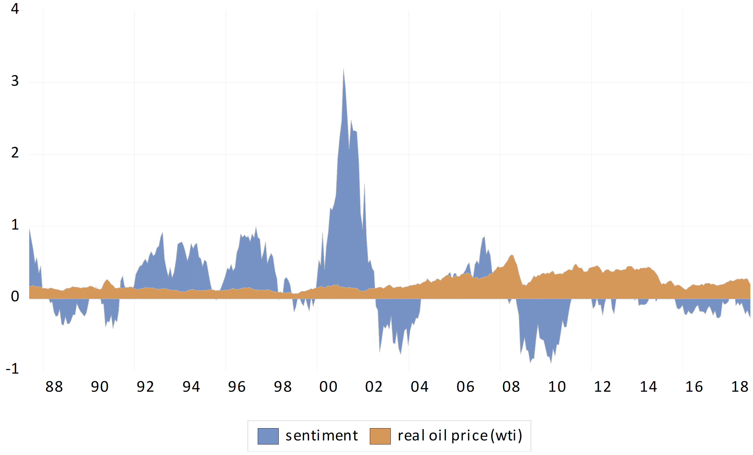
We employ monthly data from May 1987 to December 2018. Oil price (roilp) is measured by the West Texas Intermediate (WTI) crude oil price. Prior to analysis, the WTI crude nominal oil prices are deflated by using monthly constant Consumer Price Index data from the United States, with 2015 as the base year, to obtain real oil prices. We use WTI in the analysis because it is a benchmark for the US oil market. Data on oil prices and the Consumer Price Index are retrieved from the Federal Reserve Bank of St. Louis website. For investor sentiment (sent), we use the investor sentiment index developed by Baker and Wurgler (2007). It is constructed by the first principle component of six factors: the dividend premium, the number of initial public offerings, these offerings’ first-day returns, the New York Stock Exchange share turnover, the closed-end fund discount, and the share of equity issues in total debt and equity issues. Figure 1 plots real oil prices and investor sentiment from May 1987 to December 2018.

Fig. 1.Real oil prices (WTI) and investor sentiment

This graph shows the behavior of real oil prices (WTI) and investor sentiment from 1987m5 to 2018m12.

III. RESULTS

We start the analysis by testing the stationarity of the variables using the Phillips–Perron (PP) (1988) unit root test. The results reported in Table 1 show that $sent_t$ is I(0), and the rest of the variables are I(1).

Panels a and b of Fig. 2 present the recursive evolving homoskedasticity and heteroskedasticity results, respectively. The recursive evolving homoskedasticity test results show that there is solid bidirectional causality between oil prices and sentiment, suggesting that oil prices and sentiment mutually influence each other. On the other hand, the recursive evolving heteroskedasticity-consistent test results reveal that oil prices Granger-cause sentiment only in the periods May 1987 to May 1993, November 1993 to March 1994, and June 1994 to December 2018, while investor sentiment Granger-causes oil prices in all periods, suggesting strong Granger causality from investor sentiment to oil prices.

Fig. 2.Recursive evolving Granger causality between investor sentiment and real oil price

This graph shows recursive evolving Granger causality between investor sentiment and real oil price (Homoskedasticity and heteroskedasticity Wald statistics). — denotes the test statistics sequence; - - - - and …. denote 10% and 5% critical value sequence, respectively. The lag augmentation equals one (d=1). Lag orders are based on AIC with a maximum length of 8 for the sample.

Table 2 reports the recursive evolving time-varying causal relation between positive and negative changes in oil prices and investor sentiment under different error assumptions (homoskedasticity and heteroskedasticity, respectively), and Figs. A1 and A2 in the Appendix respectively illustrate it. For example, the homoskedasticity results reveal that positive shocks in sentiment Granger-cause positive changes in oil prices only during the three periods of October 1993 to December 1993, March 1994, and April 1995 to December 2018, while positive changes in oil prices Granger-cause positive changes in investor sentiment for the whole period. When it comes to heteroskedasticity-consistent results, positive changes in investor sentiment Granger-cause positive movements in oil prices from January 1995 to December 2018, while positive changes in oil prices Granger-cause positive movements in investor sentiment in all periods.

IV. CONCLUSION

This study assesses the causal relation between investor sentiment and oil prices in the United States. We find bidirectional causality between investor sentiment and oil prices using macro-level data at the monthly frequency from May 1987 to December 2018 and a newly developed time-varying causality approach. Our findings emphasize the interdependencies between investor sentiment and oil prices and speak to both investors and the oil market. For future study, other proxies of investor sentiment can be used to investigate investor sentiment–oil price causality.

Appendix

Fig. A1.Recursive evolving Granger causality between investor sentiment and real oil price

This graph shows the recursive evolving Granger causality between investor sentiment and real oil price based on homoscedastic Wald statistics. — denotes the test statistics sequence; - - - - and …. denote 10% and 5% critical values, respectively. The lag augmentation equals one (d=1). Lag orders are based on AIC with a maximum length of 8 for the sample.

Fig. A2.Recursive evolving Granger causality between investor sentiment and real oil price

This graph shows the recursive evolving Granger causality between investor sentiment and real oil price based on heteroscedastic Wald statistics. — denotes the test statistics sequence; - - - - and …. denote 10% and 5% critical values, respectively. The lag augmentation equals one (d=1). Lag orders are based on AIC with a maximum length of 8 for the sample.