I. Introduction

The debate over whether crude oil in different countries or locations constitutes a unified world oil market is still ongoing. China is the world’s largest importer of crude oil and is second in oil consumption. On March 26, 2018, China launched renminbi-denominated crude oil futures on the Shanghai International Energy Exchange (INE). The INE crude oil futures market is the first Chinese derivatives market open to international traders, particularly in the Asia-Pacific region. Although INE has been trading for three years, some argue that its prices lag behind Western price benchmarks, since it lacks a large number of international traders. To what extent these new oil futures are related to global benchmarks and whether INE has developed sufficiently to be considered an international benchmark is unclear.

The role of INE in the global oil market has been widely discussed in previous studies. Palao et al. (2020) apply a multiple regression model and find that the Brent futures market is the most influential market in the oil price discovery process, and INE has not yet altered the dominant role of Brent or West Texas Intermediate (WTI). However, Yang et al. (2020) suggest that INE crude oil futures prices can effectively reflect the fundamental information of spot markets. Evidence of Granger causality supports the efficiency of INE in the Asia-Pacific region. Since the outbreak of COVID-19 at the end of 2019 has had a big impact on crude oil prices (Narayan, 2020), it is worth exploring the changing relations between different crude oil futures prices under the influence of the pandemic.

In this paper, we investigate the dynamic correlations between Shanghai oil futures prices and global crude oil futures benchmarks. We use the daily returns of Shanghai oil futures prices and Brent oil and WTI oil futures prices for this empirical study. Following Patton (2013), we estimate the dynamic copula model, where the time-varying correlation is implemented by a generalized autoregressive score (GAS) model. Both a skewed t distribution and an empirical distribution are considered for the marginal distribution, and the GAS Student’s t copula dependence is estimated. We find dynamic correlations between Shanghai crude oil prices and international crude oil futures prices, which the COVID-19 outbreak has significantly strengthened.

Our study makes several contributions to the oil futures literature and has important policymaking implications for regulators and investors. First, different from Palao et al. (2020) and Yang et al. (2020), who focus on oil pricing efficiency, we provide new evidence about INE’s role in the global market by studying the relation between INE and global oil futures prices. Second, the dynamic correlations between Shanghai oil prices and global benchmark prices are identified. Finally, previous studies on the Shanghai oil futures (Palao et al., 2020; Yang et al., 2020) do not take into account the impact of the COVID-19 pandemic on the global oil market. We identify the significant impact of the COVID-19 pandemic on increasing the correlations of oil futures prices in different markets.

The remainder of the paper is organized as follows. Section II discusses the data and introduces the modeling approach. Section III discusses the empirical results. Section IV summarizes the main findings and draws concluding remarks.

II. Data and Methodology

A. Data and variables

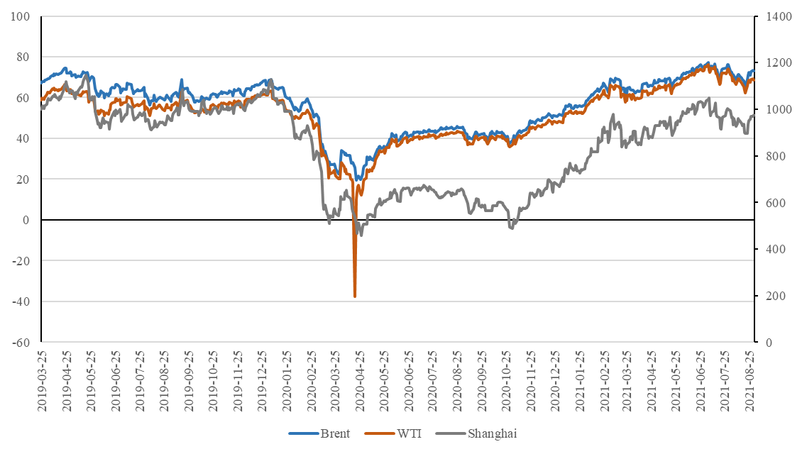
We obtain the crude oil futures of INE, Brent oil prices, and WTI oil prices from the Wind database. Our data contains 635 observations from March 25, 2019, to August 31, 2021. Figure 1 shows that Brent and WTI crude oil prices move in almost the same direction, except during the period of WTI’s collapse in April 2020. Shanghai crude oil prices (the y-axis on the right) as a whole move in much the same direction as Brent, but not as closely as WTI and Brent. Shanghai crude oil prices, as well as Brent and WTI crude oil prices reach their lowest level in April 2020, after the COVID-19 outbreak, and have since risen steadily to recover their pre-outbreak levels.

Figure 1.Oil future prices of Brent, WTI, Shanghai

This figure shows the daily prices of Brent, WTI and Shanghai oil futures. The Y-axis on the left is Brent and WTI oil futures prices, and the Y-axis on the right is Shanghai oil futures prices.

B. Methodology

The copula model is widely used to study correlations between financial data because of its flexible mathematical characteristics. Student’s t copula is better than the Gaussian copula in terms of modeling extreme events, and it captures the tail dependence between different underlying assets well. Further, the GAS model can capture time-varying correlations well. This method is widely used to estimate dynamic correlations in financial time series data (Bernardi & Catania, 2019; Lucas et al., 2019) and is often used in the commodity futures market (e.g., Ouyang & Zhang, 2020).

In this study, the time-varying copula correlations are estimated by using the Student’s t copula combined with the GAS model. First, we model the marginal distribution. We calculate the logarithmic return of oil futures prices, and we assume that it follows the following stochastic process:

$$r_{k, t} = \mu_{k, t}(X_{t − 1}) + \sigma_{k, t}(X_{t − 1})z_{k, t}, k = 1, 2,\tag{1}$$

where $X_{t - 1}$ denotes the latent underlying state vector and $z_{k,t}$ is a standardized random variable.

Second, we consider both the parametric and nonparametric marginal distributions of $z_{k,t}$. For the parametric marginal distribution, we assume that $z_{k,t}$ follows a skewed Student’s t distribution. For the nonparametric marginal distribution, we assume that the empirical distribution function is the consistent estimate of the probability distribution.

Then, we calculate the joint probability distribution of the two variables by applying the copula function $C$ (Sklar, 1959), as follows:

$$F(z_{1,t},z_{2,t} )=C(u_{1,t},u_{2,t} ),\tag{2}$$

where $u_{k,t} = F_{k}\left( z_{k,t} \right)$ and C ${\lbrack 0,1\rbrack}^{2} \rightarrow \lbrack 0,1\rbrack$ is a two-dimensional copula. We select the multivariate Student’s t distribution as our copula:

$$\begin{align}C\left( u_{1,t},u_{2,t} \right) =& \int_{- \infty}^{t_{\upsilon}^{- 1}(u_{1,t})} \int_{- \infty}^{t_{\upsilon}^{- 1}(u_{2,t})}\biggl\{\biggl\lbrack{\Gamma\left( \frac{\upsilon + 2}{2} \right)}\biggr\rbrack \\& \div \biggl\lbrack\Gamma\left( \frac{\nu}{2} \right)\sqrt{{(\pi\nu)}^{2}|\Sigma_{t}|} \\&\times \left( 1 + \frac{x'\Sigma_{t}^{- 1}x}{\nu} \right)^{- \ \frac{\nu + 2}{2}}dx_{2}dx_{1}\biggr\rbrack\biggr\} ,\end{align}\tag{3}$$

where $t_{\upsilon}^{- 1}$ is the quantile function of a standard univariate $t_{v}$ distribution and $\Sigma_{t}$ is the correlation matrix

$$\Sigma_{t} = \begin{bmatrix} 1 & \delta_{t} \\ \delta_{t} & 1 \\ \end{bmatrix}.\tag{4}$$

Next, we transform the correlation parameter $\delta_{t}$ as follows:

$$f_t=h(\delta t)\Leftrightarrow\delta_t=h^{-1}(f_t),\tag{5}$$

where $\delta_{t} = (1 - \exp\left\{ - f_{t} \right\})/(1 + exp\{ - f_{t}\}$).

Finally, using the GAS model, we calculate the correlation matrix $\Sigma_{t}$ as follows:

$$f_{t + 1} = \omega + \beta f_{t} + \alpha I_{t}^{-\frac{ 1}{2}}s_{t},\tag{6}$$

where $\omega$ denotes a constant, $I_{t}^{\frac{- 1}{2}}s_{t}$ is the score of the copula likelihood, $I_{t}: = E_{t - 1}\left\lbrack s_{t}s_{t}^{'} \right\rbrack$, and $s_{t}: = \frac{\partial\ln{c(u_{1,t},\ u_{2,t};\ \delta_{t})}}{\partial\delta_{t}}$.

III. Empirical Results

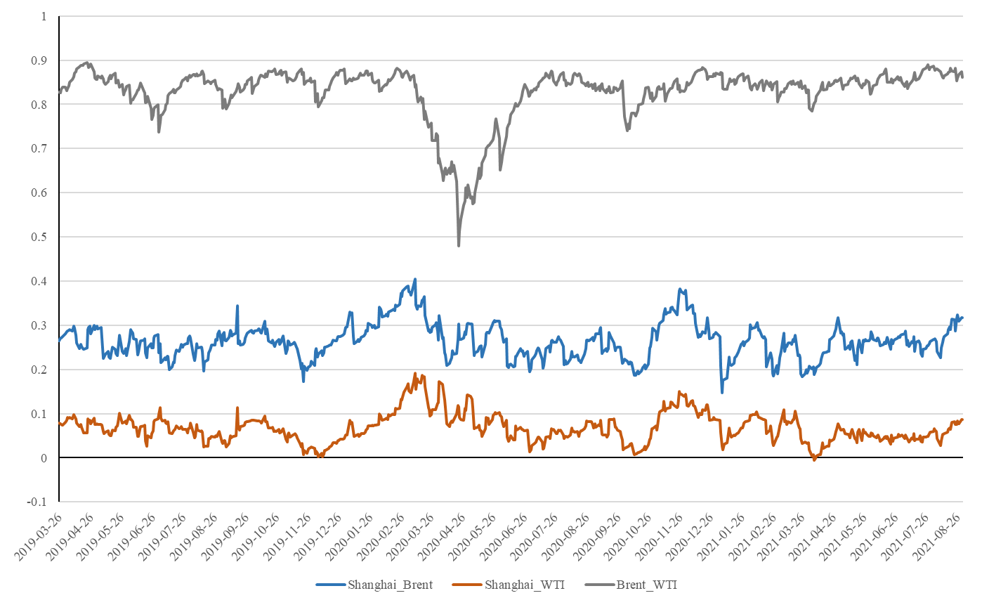
The empirical results in Table 1 suggest that the skewed t distribution outperforms the empirical distribution. Therefore, in the following copula correlation analysis, we use the GAS t copula correlations with skewed t marginals. From Table 2, we can see that the correlation between Brent and WTI is very high, reaching 0.8285. Meanwhile, the correlation between Shanghai and WTI is the lowest, with an average of 0.0687, and a maximum of no more than 0.2. The correlation between Shanghai and Brent is slightly higher than that of WTI, at 0.2642.

Figure 2 shows the dynamic copula correlations estimated by the GAS t copula. The correlation between different crude oil futures prices is time varying. The correlation between Brent and WTI has always been high, fluctuating between 0.8 and 0.9 throughout our sample period. However, the COVID-19 pandemic has had a significant impact on oil futures prices. For example, in April 2020, during the initial COVID-19 outbreak in the United States, the correlation between Brent and WTI drops sharply, even below 0.5. The correlation between Shanghai crude oil prices and international crude oil benchmarks falls to its lowest point in history at the end of 2019. Specifically, its correlation with Brent oil drops below 0.2, and its correlation with WTI drops to close to zero. However, after the COVID-19 outbreak, in January 2020, the correlation between Shanghai crude oil prices and international prices increases significantly, peaking around March 2020. As the pandemic in China is effectively brought under control, the correlation between Shanghai crude oil prices and international crude oil prices gradually drops. Then, in the fall and winter of 2020, with the second wave of COVID-19, the correlations among oil futures prices increase again.

Figure 2.Dynamic relationships between oil futures

This figure shows the GAS t copula correlations between oil futures prices from March 25, 2019, to August 31, 2021.

Our findings suggest that the correlations between Shanghai crude oil prices and international crude oil prices are not high, except during COVID-19 outbreaks. This could be due to the following reasons: first, INE trades medium sweet crude oils, a different grade of petroleum compared to Brent and WTI (light sweet crude oils). Second, the relative scarcity of international traders in Shanghai partly explains the trend. INE data show international investors accounting for just 20% of daily trades, on average, throughout 2020. Third, international investors have shied away from Shanghai crude, because trade is denominated in yuan, which carries a high risk of exchange rate fluctuation, partly due to state controls.

IV. Conclusion

In this paper, we estimate the dynamic copula model where time-varying correlations are captured by the GAS model. Both the skewed t distribution and the empirical distribution are considered for the marginal distribution. The estimated GAS Student’s t copula suggests that the correlations between Shanghai oil prices and Brent and WTI are weak but time varying. The dynamic correlations between them reach their lowest point before the outbreak of COVID-19, then rise gradually to their highest point as the outbreak begins, and afterward fluctuate continuously.

The empirical evidence suggests that, although the relations between Shanghai oil futures prices and global benchmarks have increased significantly in the short term after the pandemic, in the long term, for a variety of reasons—such as different grades of petroleum, the lack of international traders, and foreign exchange risk—INE remains a local market rather than an international benchmark.