I. Introduction and Background

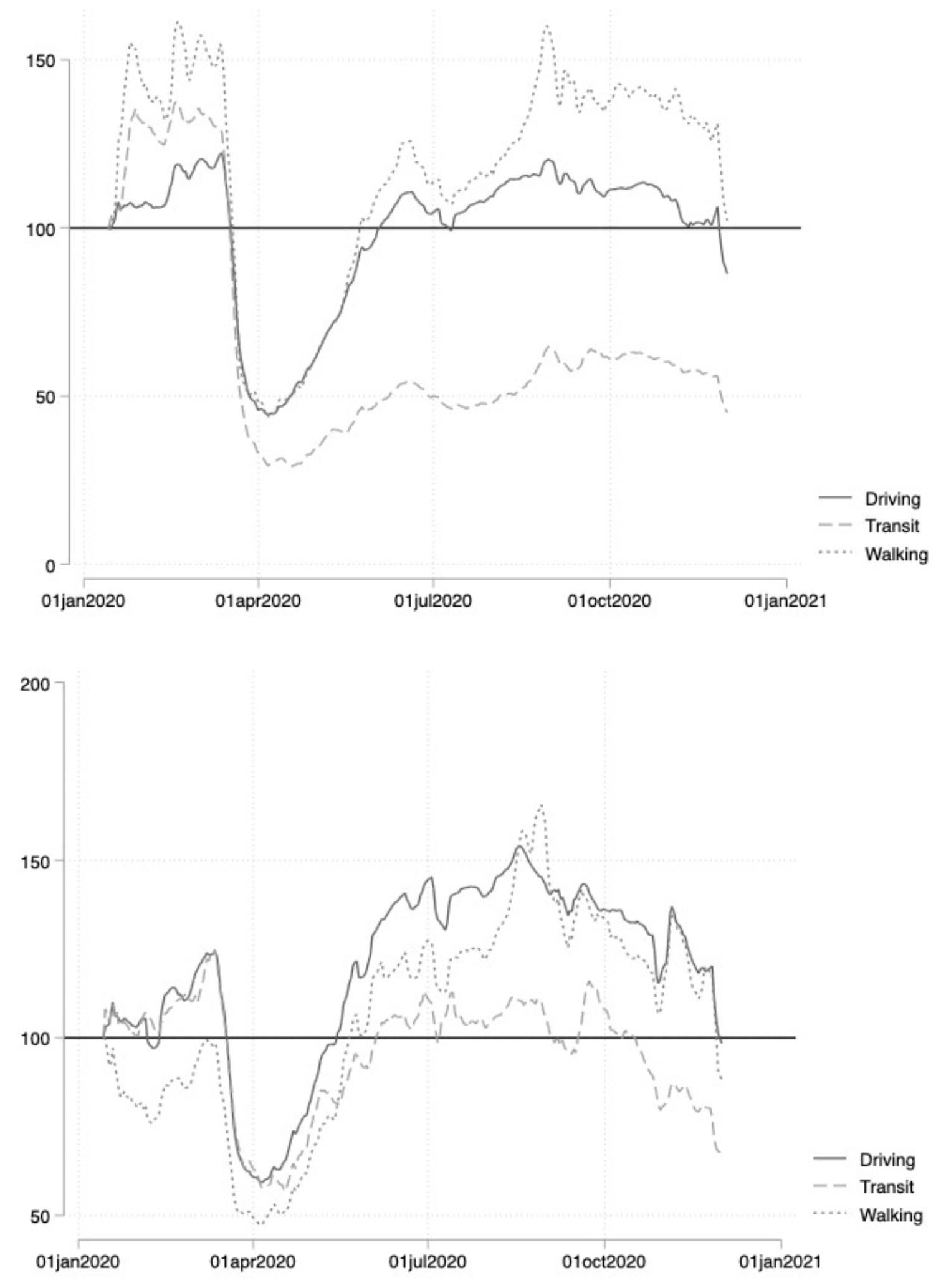
In 2020, a year in which movement was hampered by both the risk of catching COVID-19 and policies restricting travel to limit its spread, Americans still consumed more than 322 million gallons of gasoline per day. This was partly because the individual risk of spread is much lower in solitary transportation than in public transportation. How this change in the composition of travel demand ultimately affected gasoline pricing is not immediately apparent, however. On the one hand, the pandemic could have increased firms’ market power because substitutes for public transportation and other modes of transportation were severely limited. Figure 1 shows evidence of just such substitution occurring. On the other hand, retail firms often price gasoline as a loss leader to drive in-store sales. Indeed, Barron et al. (2008) find that gas station–level price elasticities are between -3 and -6. In the face of decreased demand for in-store purchases, this behavior could have been exacerbated.

Figure 1.Transportation Choices in Austin (top) and Oklahoma City (bottom)

Notes: This figure shows how transit choices have changed by mode of transportation for two cities from our sample: Austin, TX and Oklahoma City, OK.

In this paper, we use a novel data set of daily retail gasoline averages for 119 U.S. cities to determine how price markup behavior changed. The retail price series are derived from daily averages collected from user-reported prices at gas stations across select U.S. cities through the website GasBuddy. This unique data source thus captures the quick-changing price environment in each city.

It will take decades to fully account for how the pandemic shifted markets. Early analyses have started to untangle this knot using innovative data products such as cell phone tracking and Google search histories. Goolsbee and Syverson (2021) show that fear, not lockdown policies, influenced peoples’ mobility through the pandemic. Using cell phone location data, these authors find that consumer traffic fell by up to 60%, with most reductions in mobility occurring before any stay-at-home policies were issued. In the model that follows, we account for this behavior by including the rate of change in COVID-19 cases by county. The ability for jobs to be moved online was also a major factor affecting gasoline and public transportation demand. Dingel and Neiman (2020) find that approximately 37% of all jobs could be performed at home. This, of course, will affect gasoline demand across cities based on their preexisting industry makeup. We account for this using standard panel data methods and by toggling the inclusion of state-specific trends and fixed effects. We ultimately find that price–cost margins increased during the pandemic at retail gasoline stations. Given the coincidence of this change in pricing behavior with deepening unemployment and generally weak labor markets, consumer burden was likely affected very negatively. Indeed, if this change in competitive pricing is more widespread than the retail gasoline sector, then the accumulating effects certainly eroded the spending power of macroeconomic stimulus and other stabilization policies.

II. Empirical Model

We begin by calculating a city-wide metric for the competitiveness of the retail gasoline sector that is based on the classic inverse elasticity rule, or Lerner index. This measure is

$$\frac{P_{it} - MC_{it}}{P_{it}} = \frac{1}{\left| E_D \right|} \tag{1}$$

where P_it is the average retail price across stations in city i on day t, and MC_t represents the marginal cost of production. For the marginal cost, we use wholesale gas prices that are specific to retail gasoline, namely, the reformulated gasoline blendstock for oxygenate blending (RBOB) price.

Cost pass-through depends on the intensity of competition (or lack thereof). Weyl and Fabinger (2013) provide a comprehensive analysis of its incidence under imperfect competition. They show that higher competition will lead to the lower pass-through of costs, and vice versa. Higher markups typically imply higher market concentration and make it easier for firms to allow through cost shocks (but not necessarily savings).

Empirically, industry-wide studies estimating cost pass-through cover many products, from processed cheese (Kim & Cotterill, 2008), beef (Fousekis et al., 2016), and coffee (Nakamura & Zerom, 2010) to gasoline (Borenstein et al., 1997; Marion & Muehlegger, 2011; Noel, 2015). The studies are also diverse in their estimates of cost pass-through. Leibtag et al. (2007) report rates of pass-through to retailers in the US coffee market between 14% (short run, same quarter) to 59% (long run, after six quarters). Borenstein et al. (1997) estimate similar rates to those of the US gasoline market, with a rate of pass-through to retail prices of 55% (first two weeks) to 81% (after 10 weeks) following an increase in the crude oil price.

It is unclear how competitive behavior and cost pass-through will change, because the COVID-19 pandemic stands to impact retail gasoline markets in two contrasting ways: i) via an increase in demand, because consumers are choosing individual modes of transportation over public transportation, and ii) via a decrease in demand because the scale of people driving has fallen due to work-from-home policies and a general decrease in movement to entertainment and leisure venues. As an example, Figure 2 shows how daily gasoline price averages and the wholesale price of retail gasoline (RBOB) have changed in Tulsa, OK, Jacksonville, FL, and Rochester, NY. The former two cities exhibit a phenomenon known as Edgeworth price cycling, and average prices in the latter city indicate that stations use a cost-plus-fixed-fee approach to pricing. Despite the volatility, Edgeworth price cycling results in lower prices than in cost-plus-fixed-fee pricing (Noel, 2015).

A. Data

GasBuddy is a commercial website that publishes pricing data for individual stations across the United States. These prices are aggregated over many U.S. cities and published in their historical price charts with a daily resolution. Our data are gathered from digitized historical price charts from GasBuddy for 119 cities across the United States from January 1, 2019, through December 1, 2020. We couple this information with wholesale gas prices specific to retail gasoline, namely, the RBOB price.^[1] RBOB is the primary motor gasoline blending component intended for blending with oxygenates that produces the finished reformulated gasoline sold at retail locations.

The cities in our sample were selected because they coincide with those whose data on changes in mode of transportation are covered in the Apple COVID-19 mobility data reports. These data are built on changes in requests for directions gathered by the Apple Maps app.^[2] Figure 1 shows how transportation choices changed in Austin, TX, and Oklahoma City, OK. We also gather data on the amount of new COVID-19 cases reported at the county level for each city in our sample from a common repository available through The New York Times.^[3]

B. Model

Our primary model is

$$\begin{align} Lerner_{it} = &= \beta_0 + \beta_1 \Delta \ln \left( Cases_{it} \right) \\ &+ \beta_2 Transit_{it} + \beta_3 March_t \\ &+ \beta_4 April_t \\ &+ \sum_{s=0}^n \left( \pi_0 + {}_i I \left( State_s \right) * \lambda_t \right) \\ &+ \gamma_i + \lambda_t + \varepsilon_{it} \end{align} \tag{2}$$

where the dependent variable, Lerner_it, is the Lerner index for city i on day t. Our coefficient of interest is β₁, which captures the effect of a 1% change in COVID-19 cases on the Lerner index, all else being equal. This measure is calculated as the logarithm of the difference of the seven-day moving average of cases for each city. We control for outside transportation options by including Transit_it, which is the seven-day moving average of the transit index for each city. The variables March_i and April_i are dichotomous indicators for March and April of 2020, which are widely recognized as the first two months of the pandemic.^[4] These are the months in which the price–cost index was the most volatile, since various stay-at-home policies were being enacted and uncertainty was extremely high.

The bottom row of variables includes city and weekday fixed effects (γ_i and λ_t, respectively) which control for unobservable time-invariant differences in markups that are specific to each city or day of transit. We also toggle the use of state-specific trends and state-specific period fixed effect variables. Our state-specific variables account for nonlinear aggregate shocks to markups that are common across all cities within a state (e.g., state policies on working from home, which businesses are allowed to be open, and even masking policies). Our identification of the effect of new COVID-19 cases on retail gasoline markups relies on conditional exogeneity. Conditional on available transportation choices, city, day, and state-specific fixed effects in the model, any remaining impacts on markups are likely random.

Figure 2.Price histories for Tulsa (top), Jacksonville (middle) and Rochester (botttom)

Notes: This figure shows how retail prices and wholesale (RBOB) prices have changed over time in three cities from our sample: Tulsa (top), Jacksonville (middle) and Rochester (bottom). In each figure the average retail price is shown with a solid line, and the RBOB price is shown with a dotted line.

C. Results

Table 2 shows our results. Column 1 includes no fixed effects or state-specific variables, column 2 adds fixed effects, and columns 3 and 4 toggle between the inclusion of state-specific linear trends and state-specific period fixed effects. Across all models, we find that increases in the growth rate of new COVID-19 cases increase the price–cost margin represented by the Lerner index. The mean Lerner index value in our sample is 0.336. This result is consistent with a station-level elasticity of demand of approximately -3, which is in line with the findings of Barron et al. (2008), who were able to toggle station prices at 54 different locations in major Californian cities and observe the reactions of market competitors. In our preferred specifications, we find that a 10% increase in new COVID-19 cases is associated with a 0.33 change in the Lerner index. Relative to the mean, this is tantamount to the station-level elasticity of demand changing from -3 to about -1.5, a much less competitive environment than before the pandemic or that prior research would suggest.

Holding constant changes in new COVID-19 cases, we also find that price-cost margins decrease as public transit increases. This effect is rather small in magnitude, though.^[5] Finding that more public transportation reduces the Lerner index makes intuitive sense, especially since we are able to account for local and state-to-state differences in policies with the inclusion of state by week fixed effects or state-specific trends.

III. Conclusion

In this research, we investigate how competitive pricing has been impacted by the COVID-19 pandemic. To do so, we focus on the retail gasoline sector using daily pricing data for 119 cities in the United States. Historically, competition across stations is intense, because prices are very visible, and city-wide price information is salient to interested consumers through services like GasBuddy. Ex ante, the effects of COVID-19 and policies meant to limit its spread on competition and gasoline price markups are unclear, because mobility and demand broadly decreased through income effects, but risk-free transportation options were severely limited, which could drive new demand to gas stations. We find that new cases of COVID-19 are associated with an increase in the Lerner price–cost index. This means that retail gasoline markets became less competitive due to the spread of COVID-19. Given these competitive effects, we expect that new costs would pass through more quickly to consumers and that cost savings would be slower to pass through to prices. Given the coincidence of this change in pricing behavior with deepening unemployment and generally weak labor markets, the consumer burden was likely very negatively affected. Indeed, if this change in competitive pricing is more widespread than the retail gasoline sector, then the accumulating effects certainly eroded the spending power of macroeconomic stimulus and stabilization policies.

Future welfare analyses to determine the full consumer burden effects of competitive pricing behavior during this period will be illuminating. We further believe that future research could consider other proxies for the presence of COVID-19, since we use only county case rates.