1. Introduction

Our study examines the effect of uncertainties due to infectious disease outbreaks (INF) on the energy futures market. Our study is relevant as disease outbreaks, such as the current COVID-19 pandemic, can distort economic activities, causing economic and financial uncertainties, triggering increased unemployment. These resultant consequences may lead to international financial chaos that disturbs asset allocations and risk management and, most notably, financial stability (Bouri et al., 2020). According to Qin et al. (2020), the COVID-19 pandemic had a substantial negative net effect on oil prices by as much as 80%. Similarly, the severe acute respiratory syndrome (SARS) outbreak of 2003 also had a severe effect on oil prices. However, this often-held negative assertion may change as a pandemic outbreak may trigger a negative supply shock, driving up prices (Qin et al., 2020). Therefore, a study of this nature may help investors re-stabilize their portfolios, switching from risky assets to safe-haven assets in order to mitigate portfolio risks (Bouri et al., 2020).

A few studies have attempted to explain the interaction between pandemics and financial markets. Salisu & Adediran (2020) find that the infectious disease equity market volatility is a good predictor of energy market volatility in both in-sample and out-of-sample tests. Liu et al. (2020) examine the interaction among the COVID-19 pandemic, crude oil market, and the U.S. stock market, and find a negative connection between crude oil returns and stock returns. Interestingly, they also discover that the COVID-19 pandemic cannot exert a negative effect but has a statistically significant positive effect on crude oil returns and stock returns. Mazur et al. (2020) investigate the U.S. stock market performance during the crash of March 2020 triggered by COVID-19 and find that natural gas, food, healthcare, and software stocks earn high positive returns, while equity values in petroleum, real estate, entertainment, and hospitality sectors fall significantly. The study also finds that loser stocks exhibit extreme asymmetric volatility, which correlates negatively with stock returns. However, it is still unknown to what extent uncertainties due to infectious disease outbreaks affect the energy futures markets. In theory, outbreaks of infectious diseases will restrain energy demand, leading to a decline in energy prices and returns. There is also the possibility that investors’ expectations may be affected adversely, causing a fall in stock returns (Liu et al., 2020). Since investors take different actions to deal with possible risks and uncertainties, they may choose to delay investment decisions and investments, which eventually reduce stock returns.

This paper extends the literature on COVID-19 by focusing on the causal impact of uncertainties due to infectious disease outbreaks on the energy futures market. To this end, we utilize the novel non-parametric causality-in-quantiles approach recently developed by Balcilar et al. (2016). This approach can test the non-linear causality of the kth order across all quantiles of the entire distribution of commodity returns and is robust to the presence of misspecification errors, structural breaks, and frequent outliers, which are frequently found in financial time series (Balcilar et al., 2016). Furthermore, as a justification for using the non-parametric quantile-in-causality approach, we conduct a test for non-linearity by applying the Brock et al. (1996) test which validates the adoption of the non-linear causality-in-quantiles approach.

The rest of the paper is structured as follows. Section 2 provides a description of the methodology. Section 3 presents the discussion of data and empirical results, and Section 4 concludes.

2. Methodology

This paper follows the Balcilar et al. (2016) methodology, which is an extension of the Nishiyama et al. (2011) and the Jeong et al. (2012) non-linear causality frameworks. As noted by Jeong et al. (2012), the variable $x_{t}$ (INF) does not cause $y_{t}$ (energy future returns) in the $\sigma$-quantile with respect to the lag-vector of $\{ y_{t - 1},\ldots,\ y_{t - q},\ x_{t - 1},x_{t - q}\}$ if

$$\begin{align} \hspace{10mm} Q_{\sigma}\left( y_{t} \middle| y_{t - 1},\ \ldots,y_{t - q},\ x_{t - 1},\ldots,x_{t - q} \right)& \\ \hspace{10mm} = Q_{\sigma}\left( y_{t} \middle| y_{t - 1},\ \ldots,y_{t - q} \right)& \hspace{10mm} (1) \end{align}$$

While $x_{t}$ causes $y_{t}$ in the $σth$ quantile with respect to $\{ y_{t - 1},\ldots,\ y_{t - q},\ x_{t - 1},x_{t - q}\}$ if

$$\begin{align} \hspace{11mm} Q_{\sigma}\left( y_{t} \middle| y_{t - 1},\ \ldots,y_{t - q},\ x_{t - 1},x_{t - q} \right)& \\ \hspace{11mm} \neq Q_{\sigma}\left( y_{t} \middle| y_{t - 1},\ \ldots,y_{t - q} \right)& \hspace{13mm} (2) \end{align}$$

Definitively, $Q_{\sigma}\left( y_{t} \middle| \bullet \right) = \sigma th$ quantile of $y_{t}$ depending on t and $0 < \sigma < 1.$ We denote $V_{t - 1} \equiv (y_{t - 1},\ \ldots,y_{t - q})$, $U_{t - 1} \equiv$ $\left( x_{t - 1},\ldots,\ x_{t - q} \right),$ and $W_{t} = (U_{t},V_{t})$; and $F_{y_{t}|W_{t - 1}}(y_{t}|W_{t - 1})$ and $F_{y_{t}|V_{t - 1}}(y_{t}|V_{t - 1})$ represents the conditional distribution of $y_{t}$ given $W_{t - 1}\ and \: V_{t - 1},$ respectively. Also, $F_{y_{t}|V_{t - 1}}(y_{t}|V_{t - 1})$ is assumed to be absolutely continuous in $y_{t}$ for almost all $W_{t - 1}$. If we proceed by denoting $Q_{\sigma}(W_{t - 1}) \equiv Q_{\sigma}\left( y_{t} \middle| W_{t - 1} \right)$ and $Q_{\sigma}(V_{t - 1}) \equiv Q_{\sigma}\left( y_{t} \middle| V_{t - 1} \right)$, then we have $F_{y_{t}|W_{t - 1}}\left\{ Q_{\sigma}\left( y_{t} \middle| W_{t - 1} \right) \right\} = \sigma$ with a probability of one. The hypothesis to be tested based on the specified definitions in Equations (1) and (2) are;

$$\hspace{3mm} H_{0} = P\left\{ F_{y_{t}|W_{t - 1}}\left\{ Q_{\sigma}\left( y_{t} \middle| W_{t - 1} \right) \right\} = \sigma \right\} = 1, \hspace{3mm} (3)$$

$$\hspace{3mm} H_{1} = P\left\{ F_{y_{t}|W_{t - 1}}\left\{ Q_{\sigma}\left( y_{t} \middle| W_{t - 1} \right) \right\} = \sigma \right\} < 1, \hspace{3mm} (4)$$

Following Jeong et al. (2012), the distance measure $J = \left\{ \tau_{t}E(\tau_{t} \middle| W_{t - 1})f_{W}(W_{t - 1}) \right\}$, where $\tau_{t}$ and $f_{z}(W_{t - 1}$) are the regression error and marginal density function of $Z_{t - 1}$, respectively. The regression error in Equation (3) can only be true if and only if $E\lbrack 1\left\{ y_{t} \leq Q_{\sigma}\left( V_{t - 1} \right) \middle| W_{t - 1}) \right\} = \sigma$ or, equivalently, $1\left\{ y_{t} \leq Q_{\sigma}\left( V_{t - 1} \right) \right\} = \sigma + \tau_{t}$, where $1\{ \bullet \}$ is the indicator function. Thus, Jeong et al. (2012) specify the distance measure, $G \geq 0$, as:

$$G = E\left\lbrack \left\{ F_{y_{t}|W_{t - 1}}\left\{ Q_{\sigma}\left( y_{t} \middle| W_{t - 1} \right) \right\} - \sigma \right\}^{2}f_{W}\left( W_{t - 1} \right) \right\rbrack \hspace{2mm} (5)$$

We will have a situation where $G = 0$ if and only if the null in Equation (3) is true, while we will have $G > 0$ otherwise in Equation (4). To test for the J-statistic, feasible kernel-function of Equation (6) is used:

$${\widehat{G}}_{T} = \frac{1}{T\left( T - 1 \right)s^{2q}}\sum_{t = q + 1}^{T}\ \sum_{r = q + 1,r \neq t}^{T}K\left( \frac{W_{t - 1} - Z_{s - 1}}{s} \right)\widehat{\tau_{t}}\widehat{\tau_{s}}, \hspace{2mm} \large{(6)}$$

Where $K( \bullet )$ denotes the kernel function with bandwidth s. T, q, $\widehat{\tau_{t}}$ is the sample size, lag-order and estimate of the regression error, respectively. The estimate of the regression error is computed as thus:

$$\hspace{13mm} \widehat{\tau_{t}} = 1\left\{ y_{t} \leq \widehat{Q_{\sigma}}\left( Y_{t - 1} \right) \right\} - \sigma \hspace{20mm} (7)$$

Also, we further use the non-parametric kernel method to estimate the $σth$ conditional quantile of $y_{t}$ given $V_{t - 1}$ as ${\widehat{Q}}_{\sigma}\left( V_{t - 1} \right) = {\widehat{F}}_{y_{t}|V_{t - 1}}^{- 1}\left( \sigma \middle| V_{t - 1} \right),$ where the Nadarya-Watson Kernel estimator is specified as follows :

$$\begin{align} \hspace{4mm} &{\widehat{F}}_{y_{t}|V_{t - 1}}^{\ }\left( y_{t} \middle| V_{t - 1} \right) \\ &\hspace{7mm}= \frac{\sum_{r = q + 1,r \neq t}^{T}{N\left( \frac{V_{t - 1} - V_{r - 1}}{s} \right)}1(y_{r} \leq y_{t})}{\sum_{r = q + 1,r \neq t}^{T}{N\left( \frac{V_{t - 1} - V_{r - 1}}{s} \right)}} \hspace{5mm} (8) \end{align}$$

Where $N\left( \bullet \right)$ is the kernel function and s is the bandwidth.

Balcilar et al. (2016) extend the above frameworks to account for causality in higher order moments, such that

$$\hspace{18mm} y_{t} = h\left( V_{t - 1} \right) + \vartheta\left( U_{t - 1} \right)\tau_{t}, \hspace{18mm} (9)$$

Where $\tau_{t}$ is the white noise process and $h( \bullet )$ and $\vartheta( \bullet )$ equals the unknown functions that satisfy pertinent conditions for stationarity. Although, this specification allows no granger-type causality testing from $U_{t - 1}$ to $y_{t}$, it could detect the “predictive power” from $U_{t - 1}\ to\ y_{t}^{2}$ when $\vartheta( \bullet )$ is a general non-linear function. Thus, the study re-formulates Equation (9) to account for the null and alternative hypothesis for causality in variance in Equations (10) and (11):

$$\hspace{3mm} H_{0} = P\left\{ F_{y_{t}^{2}|W_{t - 1}}\left\{ Q_{\sigma}\left( y_{t} \middle| W_{t - 1} \right) \right\} = \sigma \right\} = 1, \hspace{3mm} (10)$$

$$\hspace{3mm} H_{1} = P\left\{ F_{y_{t}^{2}|W_{t - 1}}\left\{ Q_{\sigma}\left( y_{t} \middle| W_{t - 1} \right) \right\} = \sigma \right\} < 1, \hspace{3mm} (11)$$

The feasible test statistic for testing of the null hypothesis in Equation (10) is obtained, and then replace $y_{t}$ in Equations (6) – (8) with $y_{t}^{2}$ (that is, volatility). With the inclusion of the Jeong et al. (2012) approach, the study overcomes the issue that causality in mean implies causality in variance. Specifically, the study interprets the causality in higher-order moments through the use of the following model:

$$\hspace{18mm}y_{t} = h\left( U_{t - 1},V_{t - 1} \right) + \tau_{t}, \hspace{18mm} (12)$$

Thus, we specify the higher order quantile causality as

$$\begin{align} \hspace{5mm} H_{0} = P\left\{ F_{y_{t}^{k}|W_{t - 1}}\left\{ Q_{\sigma}\left( y_{t} \middle| W_{t - 1} \right) \right\} = \sigma \right\} = 1, \hspace{2mm}& \\ for\ k = 1,2,\ldots,k, \hspace{10mm} &(13) \end{align}$$

$$\begin{align} \hspace{5mm} H_{1} = P\left\{ F_{y_{t}^{k}|W_{t - 1}}\left\{ Q_{\sigma}\left( y_{t} \middle| W_{t - 1} \right) \right\} = \sigma \right\} < 1, \hspace{2mm}& \\ for\ k = 1,2,\ldots,k. \hspace{10mm} &(14) \end{align}$$

Overall, we test that $x_{t}$ granger causes $y_{t}$ in $σth$ quantile up to the K-th moment through the use of Equation (13) to construct the test statistic of Equation (6) for each k. Although, Nishiyama et al. (2011) note that it is not easy to combine different statistics for each $k = 1,2,\ldots,k$ into one statistic for the joint null in Equation (13), which is mutually correlated. However, to circumvent this issue, we adopt a sequential-testing method as described by Nishiyama et al. (2011). To begin with, we test for the non-parametric Granger causality in mean (k=1). Failure to reject the null of k=1 does not translate into non-causality in variance, thus, we construct the tests for k=2. Finally, we test for the existence of causality-in-mean and variance successively.

3. Discussion of Results

3.1 Data and Preliminary Analyses

This paper covers four (4) different energy futures. These are; Gasoline, Heating Oil, Natural Gas, and West Texas Intermediate (WTI). We adopt daily data from January 1, 1985, to August 13, 2020. The scope and frequency of our study are based on data availability. Data on the energy futures is obtained from the Thomson Reuters DataStream. As a proxy for INF, we adopt the Infectious Disease Equity Market Volatility data developed by Baker et al. (2020) and are available for download from Baker’s website http://www.policyuncertainty.com. The returns of the series are computed as the first difference of the natural logarithm of the level series.

Table 1 highlights the relevant descriptive properties of the series. Considering the results presented in Panel A, all energy futures observe positive returns in their average values ranging between $2.08 (Gasoline) and $43.63 (WTI). However, a massive difference is observed between the maximum and minimum values of the WTI and INF, indicating susceptibility to high levels of fluctuations without the certainty of stability over time. Furthermore, the WTI standard deviation value is relatively large; this may not be unrelated to the recent severe impact of COVID-19 occurrence, implying significant outliers. Also, the skewness statistic shows that all are positively skewed. The kurtosis statistics also reveal that all series are largely platykurtic (lowly peaked) - this kind of distribution has a tail that is thinner than a normal distribution, which generally produces results that would not be very extreme. This is good news for investors who do not prefer to take a lot of risk. However, INF, on the other hand, is highly leptokurtic. The Jarque-Bera statistic also confirms non-normality. This may indicate the existence of heavy right or left tail and excess kurtosis, suggesting the presence of non-linearity and/or structural shifts along the time paths of the series. The use of linear or constant parameter models would bring about spurious results. Hence, our choice of quantiles-based causality test. Also, the existence of heavy tails and high volatility necessitates examining the relationship in both the conditional-mean and conditional-variance (see Balcilar et al., 2016). Panel B of Table 1 contains results of the augmented Dickey-Fuller (ADF) and the Phillips-Perron (PP) unit root tests; the returns series of all considered variables are found to be stationary at level.

3.2 Causality test results

We begin the analysis by examining the causal effect of INF on the returns of energy futures from a linear perspective. The results are reported in Table 2 Panel A. It is observed that INF’s effect is significant in most cases at the 10% level with the exemption of natural gas returns. This may likely be due to the presence of non-linearity in the series.

Furthermore, to nonlinearity, we conduct a more formal test (BDS test) developed by Brock et al. (1996) to establish the presence of non-linearity in the series. The BDS test results (reported in Table 2 Panel B) show strong evidence of a non-linear relationship between INF and all the return series. The null hypothesis of serial dependence is rejected at the highest levels of significance. These results imply strong evidence of non-linearity in the relationship between INF and the returns of the energy futures market. Reliance on the linear Granger-causality test may lead to spurious conclusions as it could have suffered from misspecification errors.

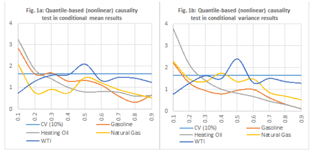
Having established non-linearity, we turn to the results of the quantiles-based causality tests. In order not to miss out on any vital information, the quantiles-based causality analysis is conducted in both the conditional-mean and conditional-variance (see Table 3), and a graphical representation is also presented in Figure 1. There is strong evidence in support of the rejection of the null hypothesis of no Granger-causality. The causal evidence is mostly significant at the lower quantiles, with some reaching the median region. However, the causality becomes weak at the extreme quantiles, suggesting that the effect of uncertainties due to infectious disease outbreaks on the returns of energy futures is sensitive to the degree of the energy futures markets’ performance. In other words, when the markets are performing at their peak, the effect of uncertainties due to infectious disease outbreaks seems weak.

Figure 1:**Quantile-based (non-linear) causality test in conditional mean and variance

Note: The above figures are graphical representations of the Causality-in-quantiles in conditional mean and conditional variance results. CV represents critical value at the 10% level, INF represents uncertainties due to infectious disease outbreaks, and the WTI represents West Texas Intermediate.

4. Conclusion

In this study, we examine the causal relationship between uncertainties due to infectious disease outbreaks and the energy futures market. We utilize the new dataset by Baker et al. (2020) and employ the non-parametric quantile-based approach. Our findings strongly support a non-linear causal relationship between uncertainties due to infectious disease outbreaks and the energy futures market, mostly at lower and median quantiles. This reflects the disturbing effects of infectious disease outbreaks, which matters to the formulations of policies seeking to achieve financial stability. Our conclusion complements the emerging literature on the vulnerability of the energy market to the uncertainty due to pandemic. As part of future research, it would be interesting to extend our analysis to energy related exchange traded funds and cryptocurrencies while accounting for the role of non-linearity and regime shifts. This will reveal whether our results carry over to cross-country financial markets and provide insights for global investors to develop better portfolio diversification benefits.