1. Introduction
Energy is a necessity for societies and its security and accessibility is a priority for policy makers. Since the 19th century, one of the main sources of energy has been oil and oil products, and the importance of energy has grown with time . Hence, movements in oil prices have been an important subject of research. All major oil price shocks, such as the rise in oil prices of the 1970s and 2000s and the oil price glut in the 1980s, have attracted research interests with the literature attempting to explain fluctuations (and hence volatility) in energy prices (Kocherlakota, 2009).
Energy consumption and production forecasts were made with special attention to oil crises and oil gluts over the last 50 years. Many econometric applications were conducted to analyze the demand dynamics of various oil products and to forecast consumption. For example, for Chinese electricity consumption forecasts, Zhu et al. (2011) proposed an integration of the moving average procedure and seasonal autoregressive integrated moving average model (SARIMA) with weight coefficients. J. Li et al. (2018), on the other hand, considered more than 20 combination models using traditional combination methods to forecast oil consumption in China. Rashid and Kocaaslan (2013) examined the relationship between energy consumption volatility and unpredictable variations in real GDP by estimating a Markov switching autoregressive conditional heteroskedasticity (ARCH) model for the UK. In addition, Z. Li et al. (2010) provided an analysis of future gasoline demand in Australia by using various models. They found that more sophisticated models do not always produce better forecasting results compared to simple models. They advised to determine the characteristics of time series data before modelling and forecasting them. Their suggestions were followed by Agrawal (2015) who employed an autoregressive distributed lag based co-integration model in order to forecast gasoline and diesel demand for India. In a similar fashion, but with a simpler model, Bhutto et al. (2017) forecasted annual gasoline consumption for Pakistan. Given this literature, one research gap is that there are no studies that examine how energy consumption volatility changes in the face of a global pandemic. This study aims to fill this gap by studying the Turkish diesel market during the recent COVID-19 pandemic.[1] In addition, we also show how the pandemic distorts the forecasting performance of models.
The fluctuations in oil prices started at the beginning of 2020 with the spread of COVID-19. Volatility in energy markets increased. We add to the understanding of energy markets by examining the effect of the COVID-19 pandemic on diesel consumption. Our paper is the first to investigate volatility dynamics of the diesel consumption in light of the global pandemic.
The purpose of this paper is to examine the effects of the COVID-19 pandemic on the Turkish diesel market and assess the performance of simple forecasting tools. To achieve this aim, we employ variants of the generalized ARCH (GARCH) models. These models allow us to investigate the disruptive effects of the pandemic on the Turkish diesel market. We find that volatility starts rising with the announcement of the first case and peaks at the end of May 2020. Even though purchases increase in the 2 days following the announcement, they then assume a steady downward trend.
The paper is organized as follows: Data and methodology are presented in section 2 and results are presented in section 3. Section 4 concludes.
2. Data and Methodology
In the empirical modeling, we use daily diesel consumption. Data cover the 01/01/2014 - 15/06/2020 period. Diesel consumption data are obtained from the Energy Market Regulatory Authority database. Descriptive statistics of the daily diesel consumption of Turkey are presented in Table 1.
The data suggest that the average and median daily diesel consumption are 48.8 and 49.2 million liters, respectively, while the maximum and minimum values are 22.3 and 6.2 million liters, respectively. The standard deviation stands at 10.01 million liters. This implies that daily diesel consumption varies a lot in our sample period. Moreover, the Jarque-Bera test rejects the null hypothesis of a normal distribution for daily diesel consumption. Negative skewness value for diesel consumption indicates left skewed distribution, whereas the kurtosis value of 3.242 indicates the fat tail characteristic of diesel consumption.
In order to ensure the stationarity condition, we employ logarithmic difference (growth rate) of diesel consumption data. We first investigate the stationarity of diesel consumption growth rate using both the conventional Ng-Perron unit root test and Zivot- Andrews (1992) structural break unit root test and found stationarity of the diesel consumption data.
For empirical analysis, in order to obtain the conditional heteroscedasticity (volatility) of the daily diesel consumption data, we limit ourselves to simple univariate models that have comparable performances with more sophisticated models as shown in the literature. We first estimate the best fit ARIMA structure for the mean equation. Next, we estimate alternative GARCH type models in order to analyze volatility dynamics of the daily diesel consumption. These models include ARCH, GARCH, Exponential GARCH (EGARCH) and Threshold GARCH (TGARCH), and the best model is determined based on information criteria and forecast performances.[2] Then, we obtain the conditional variance from the selected model as daily diesel volatility.
3. Results
After confirming stationarity, SARMA(7,7)(1,1) model is found to be the best model for daily diesel consumption according to model selection and forecast performance criteria[3],[4].
After we define the mean equation, we analyze volatility dynamics of the daily diesel consumption variable by employing alternative ARCH family models including ARCH, GARCH, EGARCH and TGARCH models[5]. We define the best volatility model by comparing the forecast performances of the models[6]. Table 1 presents the results of the alternative volatility models.
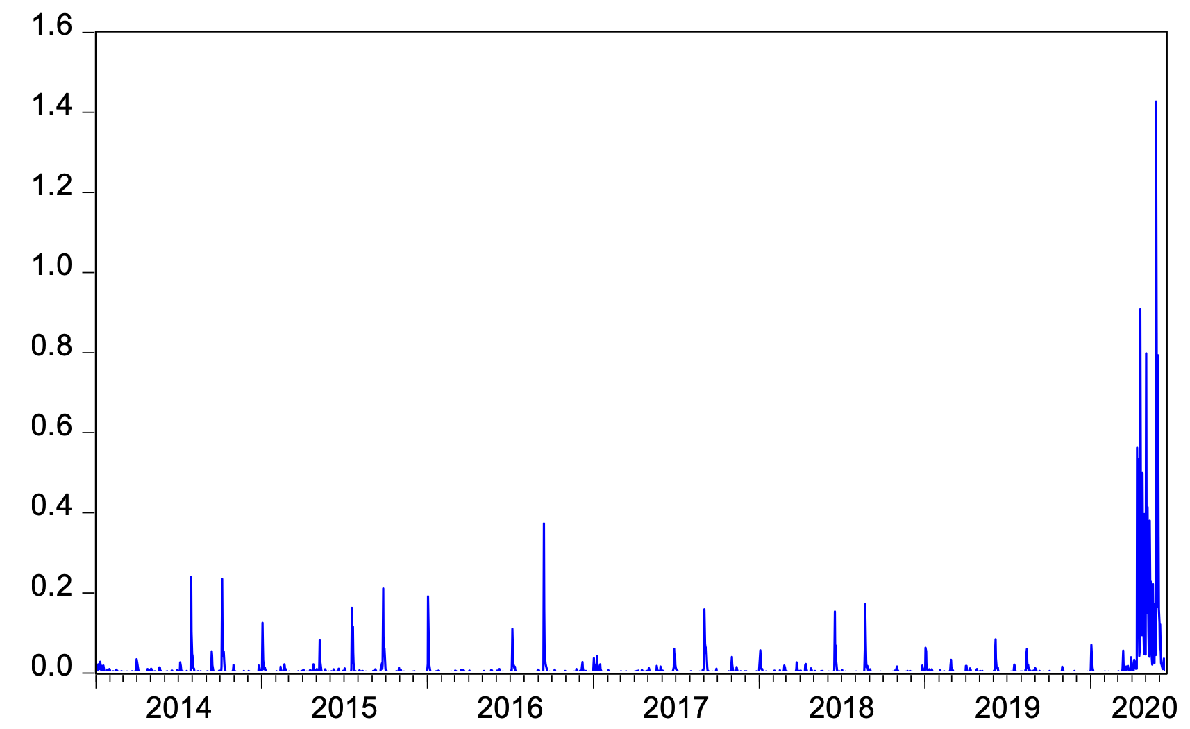
Table 1 indicates that the TGARCH(1,1) model is the best performing model according to both model selection and forecast performance criteria. The conditional heteroscedasticity of the selected model is taken as a proxy for the Turkish diesel consumption volatility. Volatility dynamics over time is presented in Figure 1.
_model.png)
As seen in Figure 1, the uncommonly high volatility starts after 11/03/2020, which is the day after of the first COVID-19 case was announced in Turkey. The volatility value reaches its peak in mid-April 2020 due to new sanctions imposed by the government, such as the weekend curfews and intercity travel restrictions. As of 11/03/2020, when the pandemic started, there was a significant increase in diesel consumption volatility. Uncertainty driven initial purchases of diesel were followed by a steady decline in consumption. Volatility reached highest levels during curfews, fell in response to normalization policies in Turkey, and converged to 0 over time.
4. Conclusion
In this note, we employ a SARMA(7,7)(1,1) model and the TGARCH(1,1) model to represent and variance of the Turkish diesel consumption. We find that a phase of high volatility starts after mid-April 2020 and peaks on 24/05/2020. A 29% decrease in diesel sales is observed between 10/03/2020 and 01/06/2020. Volatility declines after 01/06/2020 consistent with a return to normalcy. Shrinkage in the diesel market has an important adverse effect on indirect tax revenues. We make two policy suggestions to mitigate the disruption in the market. First, we suggest a temporary rearrangement of profit margins of dealers and distributors. Second, we suggest enactment of a temporary tax regulation to compensate for lost tax revenue.
COVID-19 refers to the Severe Acute Respiratory Syndrome Coronavirus 2 (SARS-CoV-2).
We kindly refer the reader to Gungor et al. (2020) for technical details of ARIMA models and volatility models.
We tried all alternative models from SARMA(0,0)(0,0) to SARMA(7,7)(1,1) that includes 256 models and defined the best 5 models according to the Log Likelihood (LogL), Akaike Information Criterion (AIC), and the Bayesian Information Criterion (BIC). The five estimated models are ARMA(7,1), ARMA(7,7), ARMA(7,6), SARMA(7,6)(1,1) and SARMA(7,7) (1,1).
Alternative ARMA model results are not presented in the text to save space. The results are available from authors upon request.
Student t distribution is used instead of a normal distribution as Jarqua-Bera test indicated non-normality.
Gungor et al. (2020) found that COVID-19 outbreak distorts the gasoline and diesel forecasts in Turkey. 10/03/2020 is the day on which the first COVID-19 case was announced. For this reason, we employ 01/01/2004 to 30/01/2020 period for model estimation and 31/01/2020 to 10/03/202 period for forecasting.