1. Introduction

Large crude oil price discounts at the wellhead, improvements in tank farm technology, and environmental concerns over flaring of natural gas have led to greater interest in crude oil pipeline development to alleviate bottlenecks and promote energy independence of the US. However, expansion of new pipeline infrastructure is not without opposition. Thus, it is important to understand the effects that crude oil pipeline takeaway capacity has on the economy. In fact, the economic impacts of pipelines on jobs, output, value added, and government revenues have been documented by Ewing and Watson (2015). As such, there is a clear link between improvements in pipeline infrastructure and the US economic performance. However, an under-researched aspect of potential benefits of pipeline infrastructure is how they impact economic stability. In light of the economic growth implications, does greater pipeline capacity lead to a more stable and less volatile economy as measured by volatility in output? This is an important question as volatility and risk are related and, accordingly, policymakers in their quest for achieving sustainable growth will benefit from knowledge regarding the relevance of pipeline capacity on growth.

The volatility of economy-wide output and industrial production is well-known (see Ewing & Thompson, 2008) and has often been examined using autoregressive conditional heteroskedasticity (ARCH) models. Notable studies include Caporale and McKiernan (1996, 1998), Speight (1999), Grier and Perry (2000), Fountas et al. (2006), Imbs (2007) and Lee (2010) to name a few. Extending this line of inquiry Ewing and Thompson (2008) looked at factors that explain the volatility of the US industrial production. There are sufficient reasons motivating why crude oil pipelines might help stabilize an economy. For instance, once installed, the ongoing operations of the pipeline transportation networks allow more efficient crude oil flow that is well-suited to respond to changes in aggregate demand, thus mitigating the business cycle. Pipeline infrastructure also relieves pressure on other forms of transportation, such as rail and truck (highway use, etc.), and enhances the supply chain by reducing what is often referred to as the “bullwhip effect”. It is along these lines that the effects of changes in pipeline capacity are considered to explain industrial production volatility and, in particular, if more pipeline capacity is associated with a more stable economy.

When both the unconditional and conditional variances of a time series, such as industrial production, is constant, then standard techniques such as ordinary least squares regression and various other time series methods apply. However, if the series exhibits ARCH, then this property violates classical regression assumptions. An ARCH-class model can predict future volatility in a series when the variance is time-varying. As noted above, US industrial production is known to follow an ARCH process. What is not known, and what is the subject of this study, is the effect that crude oil pipeline capacity has on the volatility process of industrial production.

The next section outlines the methodology and describes the data used to answer key empirical questions regarding economic stability and crude oil pipeline. A comparison of results from models with and without changes in pipeline capacity is conducted in order to address two important practical questions. For instance, does the inclusion of pipeline capacity in the volatility equation of industrial production change the persistence associated with an increase in volatility that arises from an unexpected change in industrial production (i.e. how long until things return to normal)? How and to what extent does the volatility of industrial production growth change with changes in crude oil pipeline capacity? Answers to these questions provide insight into the role that crude oil pipelines may play in economic stability. This research fills the void in the existing literature by extending the work on the economic impacts of pipelines and the results have implications for policymakers interested in sustainable economic development.

2. Empirical Results

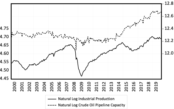
Data consist of monthly observations over January 2000-December 2019 obtained from the Federal Reserve Economic Database (https://fred.stlouisfed.gov). Industrial production (IP, Index 2012=100) represents a measure of economy-wide activity. Pipeline petroleum movement is measured in thousands of barrels and represents crude oil pipeline capacity (PC). Data are seasonally adjusted and converted to natural logs. A casual review of Figure 1 may indicate that changes in pipeline capacity are associated with periods exhibiting greater economic stability. As such, a more thorough investigation is warranted.

Figure 1:Pipeline capacity and industrial production

Note: This plots the natural log of US industrial production and natural log of crude oil pipeline capacity over time.

The first-difference of industrial production may be modeled as an autoregressive moving average (ARMA) process:

$$\varphi(L)\Delta IP_{t} = \theta(L)\varepsilon_{t} + \mu\hspace{10mm}(1)$$

where $\varphi$ and $\theta$ are polynomials in the lag operator L, and μ is a constant term. The best-fit specification was chosen based on an inspection of the autocorrelation functions and Box-Jenkins techniques. The determined model has an ARMA(2,1) specification. Consistent with previous findings (Ewing & Thompson, 2008), the Lagrange multiplier statistic (Engle, 1982) indicated the presence of ARCH effects in the first-difference of industrial production. Accordingly, the mean and variance of industrial production were estimated simultaneously using the method of maximum likelihood. The variance equation for the GARCH(1,1) model is given by:

$$h_{t}^{2} = \beta_{0} + \beta_{1}\varepsilon_{t - 1}^{2} + \beta_{2}h_{t - 1}^{2}\hspace{27mm}(2)$$
where conditional variance of ε_t with respect to the information set $\mathrm{\Omega}_{t - 1}$ is given by $V\left( \varepsilon_{t} \middle| \mathrm{\Omega}_{t - 1} \right) = h_{t}^{2}$. $\beta_{0}$, $\beta_{1}$ and $\beta_{2}$ are constant non-negative parameters and $\beta_{1} + \beta_{2} < 1$ measures volatility persistence. The restrictions on the parameters prevent negative variances and ensure that the process is covariance stationary with positive and finite variance, $\frac{\beta_{0}}{\left( 1-\beta_{1}-\beta_{2}\right)}>0$ (Bollerslev, 1986). Equation (3) is estimated in order to examine how changes in crude oil pipeline capacity impact the volatility dynamics of industrial production growth.

$$h_{t}^{2} = \beta_{0} + \beta_{1}\varepsilon_{t - 1}^{2} + \beta_{2}h_{t - 1}^{2} + {\rho\mathrm{\Delta}PC}_{t - 1}\hspace{10mm}(3)$$

The results from estimating the GARCH models with and without changes in PC are presented in Table 1. In both models, the estimated coefficients on the ARCH and GARCH terms are statistically significant and, therefore, volatility can be predicted in the presence of time-varying volatility. Also, in both cases the models are shown to be covariance stationary, that is, $\frac{\beta_{0}}{\left(1-\beta_{1}-\beta_{2}\right)}>0$.

As noted above, $\beta_{1} + \beta_{2}$ shows the degree of volatility persistence. Compared to the model without accounting for pipeline capacity, the results from the GARCH model with changes in pipeline capacity show a nearly 16% reduction in volatility persistence. From a macroeconomic standpoint this suggests a reduction in the length and/or magnitude of business cycles when considering how long volatility (a measure of cycle) lasts. Put differently, if a standardized shock would otherwise increase volatility for a period of one year (i.e., the volatility takes one year to dissipate), then a one percent increase in pipeline capacity would reduce the extent of the shock or the time it persists by nearly two full months. Further, the effect that pipeline capacity has on economic stability is shown by the negative and significant coefficient on ΔPC. The result provides evidence of a significant decline in the volatility of industrial production with increases in pipeline capacity. This finding adds to the literature on economic impacts of pipelines by showing that an additional benefit of crude oil pipeline is a more stable economy, as measured by the volatility of industrial production.

3. Concluding Remarks

Crude oil pipeline infrastructure has been shown to benefit the economy in terms of increases in jobs, output, value added, and government revenues. However, evidence as to the possible benefit of increased economic stability of pipelines has not been examined. This study documents two important findings regarding crude oil pipelines. First, the results indicate that volatility persistence of industrial production is lower with pipeline capacity included in the GARCH model than when it is excluded. As such, changes in pipeline capacity are seen to shorten the length of the business cycle. Second, including pipeline capacity in the GARCH model reduces the volatility of industrial production. Improvements in economic stability provide for a more robust, resilient and sustainable economy. Overall, the findings support the critical role that crude oil pipeline plays in the US economy.

Acknowledgement

This research was supported by a grant from ExxonMobil Pipeline Company. All opinions expressed herein are strictly those of the author. The author would like to thank the Editor and Reviewers of Energy RESEARCH LETTERS for their valuable feedback.