

I. Introduction
Rising climate change risks—such as CO₂ emissions, water scarcity, diseases, and natural disasters, pose growing threats to economies, especially financial markets (Chen et al., 2023; NguyenHuu, 2022). Natural hazards generate substantial economic losses, while transition risks arise from carbon neutrality policies. Extreme weather events disrupt operations and increase compliance costs, with heterogeneous effects across energy markets (Bua et al., 2024; Cepni et al., 2022). In 2023, EM-DAT reported approximately 400 natural hazard events globally, resulting in over USD 200 billion in damages and more than 85,000 fatalities (CRED et al., 2023).
In response, governments have implemented strategies such as promoting renewable energy, carbon taxation, emissions trading, and green finance to mitigate environmental and economic impacts (Alessi et al., 2024; Ma et al., 2024). Investors are increasingly adopting green finance instruments to hedge against climate risks while diversifying portfolios, with evidence highlighting their effectiveness in risk mitigation (Arfaoui et al., 2024; Cepni et al., 2022).
Climate risks shape renewable energy development by influencing investment and consumption (Sinha et al., 2024). Climate policy uncertainty (CPU) may encourage short-term investment in clean energy (CLE) as firms adapt to regulatory changes, yet it can constrain long-term financing for sustainable initiatives (Karlilar Pata, 2024a; Setiastuti & Rajendra, 2024). Moreover, green bonds (GB) are central to supporting the energy transition. Global green bond issuance reached USD 270 billion in 2020 (WEF, 2023) and is projected to rise to USD 1.05 trillion in 2024 (Cochelin et al., 2024).
This study investigates the dynamic relationships among clean energy, green bonds, and climate risks using a Quantile-on-Quantile approach. By analyzing the impact of natural disasters and CPU on the U.S. markets, it extends prior research, which has largely focused on CPU (Huang et al., 2025; Ma et al., 2025; Shang et al., 2022; L. Zhao et al., 2025) and provides insights for sustainable investment and policy design. This study aims to: (1) examine the dynamic relationships between clean energy, green bonds, and climate risk factors; and (2) assess the effects of ND across different quantiles on CLE and GB in the U.S. economy.
II. Data and Methodology
A. Data
The study represents clean energy with the S&P Global clean energy index and green bonds with the S&P Green Bond Index. Data for both indices were retrieved from the S&P database. Physical climate risks are measured by the financial impact of natural disasters (ND) in the U.S United States, quantified in USD, using data from the CRED database. Transition climate risks are proxied using the CPU Index, developed by Gavriilidis (2021). The data span the period from January 2, 2015, to June 9, 2023.
B. Methodology
Based on the quantile connectedness framework introduced by Chatziantoniou et al. (2021) and the work of Sim and Zhou (2015) on quantile-on-quantile regression (QQR), Gabauer and Stenfors (2024) proposed the quantile-on-quantile connectedness approach (QQC). This method aims to assess the interdependencies across different quantiles of pairs of variables. QVAR shifts its attention to the conditional quantiles of For a specific quantile the model is formulated as:
Yt=u(τ)+A1(τ)Yt−1+⋯+Aj(τ)Yt−j+ut(τ)
where and are dimensional variable vectors. The coefficients vary with the quantile enabling the relationships between variables to differ across the distribution. is the QVAR coefficient with K*K dimension, is the mean vector, is the error vector. To calculate the generalized forecast error variance decomposition (GFEVD) as outlined by Koop et al. (1996), the QVAR model is converted into a quantile vector moving average (QVMA) form:
Yt=u(τ)+P∑j=1Aj(τ)Yt−j+ut(τ)=u(τ)+∞∑i=0Bi(τ)ut−i(τ)
Following this, the F-step ahead generalized forecast error variance decomposition captures the effect that a disturbance in series j exerts on series 𝑖, expressed through the following:
∅gi←j,τ(F)=∑F−1f=0(e′iBf(τ)H(τ)ej)2Hii(τ)∑F−1f=0(e′iBf(τ)H(τ)Bf(τ)′ei)
gSOTi←j,τ(F)=∅gi←j,τ(F)∑kj=1∅gi←j,τ(F)
where measures how much shocks in series j affect the forecast error variance of series i across F-step horizons at a specific quantile (τ). is a vector of zeros, with a value of 1 at its ith element. Hii(τ) evaluates the variance of the error term for series i at a given quantile (τ). represents the scaled GFEVD. This scaled GFEVD is crucial for assessing connectedness, enabling the computation of total directional connectedness, both “TO” and “FROM” other series. The “TO” total directional connectedness shows the influence of series 𝑖 on all other series.
Sgen,toi→⋅,τ=k∑k=1,i≠jgSOTk←i,τ
The “FROM” total directional connectedness reflects the effect that all other series exert on series 𝑖.
Sgen,fromi←⋅,τ=k∑k=1,i≠jgSOTi←k,τ
The adjusted total connectedness index (TCI) measures the overall level of interdependence within a system and is expressed as follows:
TCIτ(F)=KK−1K∑k=1Sgen,fromk←⋅,τ≡TCIτ(F)=KK−1K∑k=1Sgen,tok←⋅,τ
A direct quantile relationship links high (low) quantiles of X with high (low) quantiles of Y, while an inverse relationship links high quantiles of X to low quantiles of Y. The Total Connectedness Index (TCI) measures overall interdependence, with higher values indicating stronger spillovers. TCI captures how cross-market connections change under varying and extreme market conditions.
III. Empirical Results
Figure 1 illustrates the average dynamic connectedness among CLE, GB, and climate risk factors. Stronger bidirectional links occur at inversely related quantiles, particularly between natural disasters and clean energy, with the highest TCI at the 5% ND and 95% CLE quantiles. GB shows similar patterns, while middle quantiles exhibit low connectedness. In the U.S., climate risks and green assets are more interconnected under extreme market conditions, reflecting time-varying, condition-dependent spillovers, consistent with Pham & Nguyen (2022).
At medium quantiles, representing neutral market conditions, climate risk factors exhibit minimal connections with CLE and GB, highlighting their hedging potential. Figure 1 shows the highest TCI of 46.9 at the 95th percentile of clean energy and the 5th percentile of natural disasters, with GB displaying a similar pattern. Both markets have comparable average TCIs (~30.2), though GB shows lower connectedness at inverse quantiles, indicating greater resilience. Connectedness increases at low climate risk quantiles, reflecting bear market correlations. CLE provides stronger hedging in directly related quantiles, while smaller green firms are more sensitive to policy changes, affecting returns and volatility. Green stocks support portfolio diversification and climate risk hedging (X. Zhao et al., 2022).
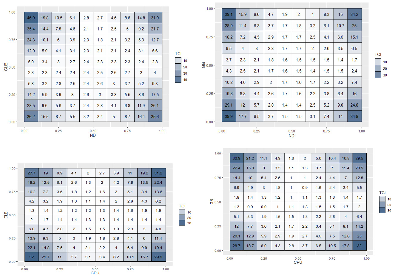
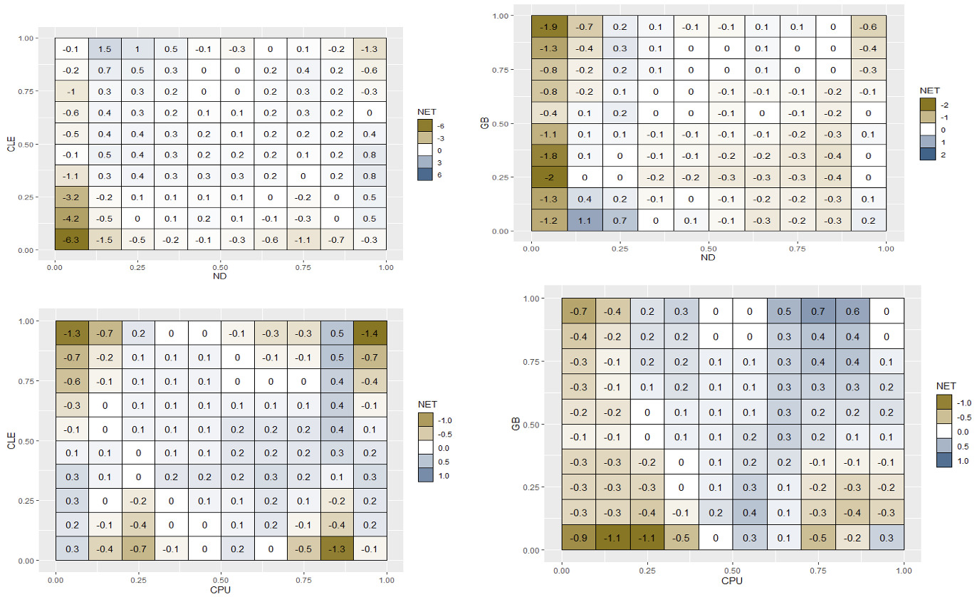
Figure 2 illustrates net directional connectedness among the variables. CLE is primarily influenced by ND, showing a mostly positive net TCI, while GB are generally net receivers from ND, except at extreme quantiles. Inversely related quantiles dominate CLE, physical risk and GB–transition risk links, indicating asymmetry. Both GB and CLE effectively hedge climate risks, attracting stability-seeking investors. Under high CPU, GB become net transmitters, reflecting conditional risk dynamics. Physical risks consistently impact CLE, while supportive policies channel investment into GB, though investor preferences shift under rising uncertainty.
Girgibo et al. (2024) highlight that climate change drives financial losses in the energy sector, while extreme weather events disrupt supply chain reliability (Xue et al., 2022). CPU may discourage investment in renewable energy, favoring cheaper fossil fuels (Meo et al., 2024). Conversely, climate risks also promote renewable energy adoption and public awareness. Governments support the transition to clean energy through measures such as carbon pricing and subsidies, and policy ambiguity can accelerate the shift toward low-carbon sources (Karlilar Pata, 2024b). Thus, climate risks simultaneously pose challenges and stimulate the low-carbon energy transition.
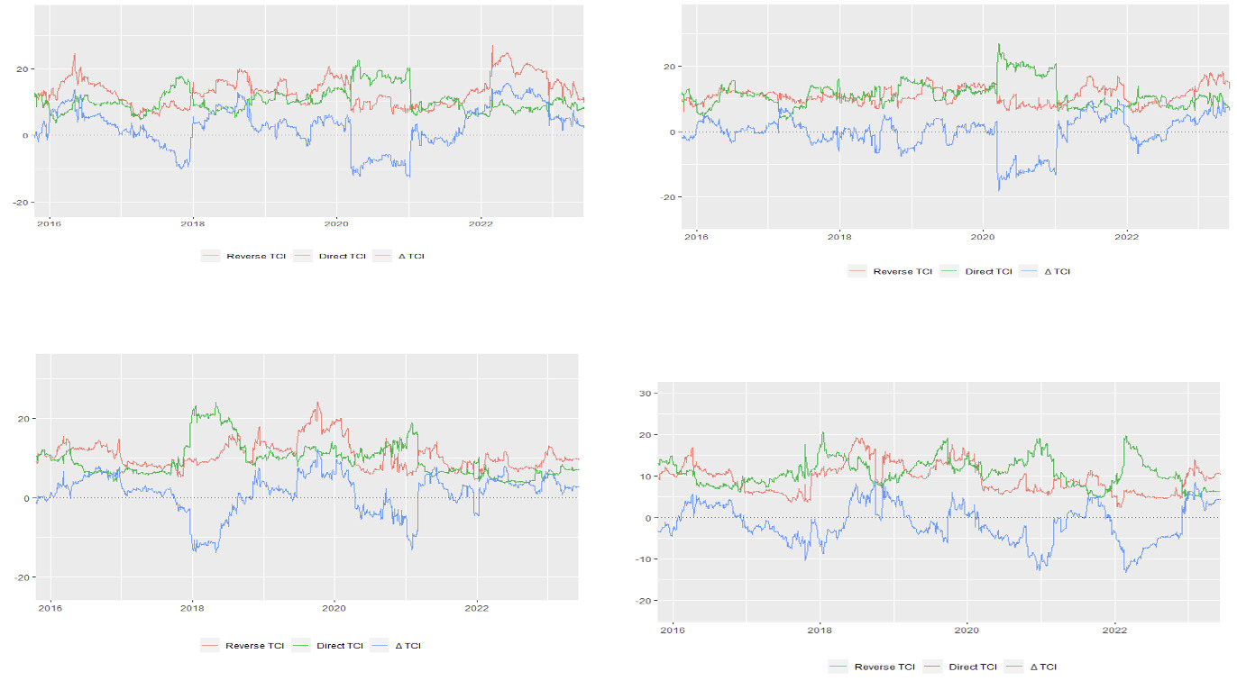
Examining direct and inverse connectedness highlights risk mitigation during market volatility. The GB-CPU relationship is mainly inverse, with a short positive peak in early 2018. CLE-ND inverse quantiles prevail between early 2016 and late 2017, early 2018 and early 2020, and pre-2022 through mid-2023, while direct TCI peaks in early 2020 amid COVID-19. After the pandemic, CLE-ND turns positive, GB-ND rises then declines, and CLE-CPU is positive from early 2017 to mid-2018 and post-COVID, but generally negative.
GB negatively correlate with transition risk, hedging CPU, while CLE mitigates physical risks. Investing in green sectors enhances market stability and diversifies climate risks. These relationships fluctuate due to CPU, which affects green project spending, redirects investor capital toward renewable energy, raises investment costs, and discourages financing of low-carbon projects (Shang et al., 2022; Wu & Liu, 2023).

The findings are consistent with Huang et al. (2025), showing that physical risks amplify connectedness and volatility. Both climate risks heighten market interdependence, but physical risks have stronger effects. By including U.S. physical climate risk alongside policy uncertainty, this study offers a broader view of climate impacts on green assets. While Pham & Nguyen (2022) highlighted volatility in green equity after major policy events, our results confirm green assets’ sensitivity to climate events, extending the analysis to include physical risks and their effects on clean energy and green bonds, which Pham’s study did not consider.
IV. Conclusion
This study examines the effects of physical (natural disasters) and transition (policy uncertainty) climate risks on GB and CLE using a QQC approach. Unlike prior research focused solely on transition risks, we incorporate the impact of natural disasters, revealing complex, market-specific relationships. Green assets are more effective at hedging transition risks, with green bonds mitigating policy uncertainty and clean energy addressing physical risks. Investing in green sectors enhances market stability and diversifies climate risk exposure. To strengthen green bonds’ climate mitigation potential, initiatives such as raising investor awareness, developing trading platforms, and supporting SMEs are essential, alongside increased government funding for renewable energy research and international collaboration. Despite these insights, the study is limited by its U.S.-centric focus, potential measurement issues, and QQC sensitivity to sample size. Future work could expand to other green finance instruments or conduct cross-country analyses for greater robustness and generalizability.
Funding
This work is supported and funded by the Deanship of Scientific Research at Imam Mohammad Ibn Saud Islamic University (IMSIU) (grant number IMSIU-DDRSP2504).