I. Introduction
India ranks second in world population and is expected to become the most populous by 2050, with a population of 1.7 billion (UN, 2022). Consequently, the demand for energy in the farm sector is set to grow to feed this growing population. Again, a continuous farm mechanisation process since the onset of the ‘Green Revolution’ in the mid-1960s has already initiated a shift from human and animal power as the primary energy sources to electricity and carbon-based fuels in Indian agriculture (Kumar et al., 2022). However, further farm mechanisation to meet the growing demand for food requires huge energy consumption in the form of electricity. In addition, the farm sector is also facing increasing climate change hazards that require additional energy to manage such abiotic risks. Hence, there is a need to energise the Indian farm sector and initiate judicious management of energy resources to maximise marginal returns in terms of additional output (Jha, 2013). Currently, the farm sector consumes around 21-24% of the country’s total electricity (Fosli et al., 2021). However, World Bank data estimates suggest that 6 million rural inhabitants of the country are still without electricity (World Bank, 2023).
In this context, there is a dire need to energise Indian farms to sustain them in large-scale food production. But here comes the policy debate: how best to assist them effectively. Or, to put it another way, should they be given cheap power subsidies to keep them going, or should more funds be allocated to rural electrification projects? Numerous empirical studies are critical of the power subsidy programme. They argue that farmers getting free or heavily subsidised electricity leads to massive groundwater exploitation and cropping pattern distortion in favour of water-guzzling crops (Akber et al., 2022; Fosli et al., 2021).
Besides environmental costs, these subsidies have substantial economic costs as they divert government expenditures from productive capital investments (Akber et al., 2022). The major input subsidies in the farm sector (fertiliser + power + irrigation) registered a thirteenfold increase from (₹10,910 crores) in 1980-81 to (₹1,51,321 crores) in 2018-19. On the contrary, public investment has continued to decline since the 1980s. Therefore, there is an increasing call for rationalising the input subsidies in favour of public investments. In addition, these subsidies, including power subsidies, are unequally distributed across the states and among farming groups (Akber et al., 2022). But, public investment in any form, be it irrigation, rural connectivity, storage, or rural electrification, is scale-neutral and beneficial to all sections.
All the above arguments raise a broad pertinent question on how efficiently Indian farms can be financed – whether through public investment or subsidisation of inputs. In the present context, we also try to examine the specific question of how we can energise Indian agriculture. In other words, whether the price support system in terms of power subsidy or expansion of rural electrification augments farm productivity in India. A careful analysis of this issue may contribute critically to policymaking for Indian agriculture. To our knowledge, this study is the first to address this issue.
II. Data and Methodology
A. Data
The study utilises time-series data from 1980-81 to 2020-21 to empirically estimate the effects of various public expenditures for investment purposes, input subsidies, and other economic factors on farm total factor productivity (TFP). Using TFP as a proxy for productivity (dependent variable) is justified because it provides a superior measure of farm productivity compared to crop yield or per capita agricultural GDP (Akber & Paltasingh, 2019). The Färe-Primont TFP index method (O’Donnell, 2011) was adopted for measuring TFP.[1] This method does not rely on restrictive assumptions such as returns to scale, optimizing behaviour in firms’ production technology, or price information. However, it satisfies all regularity conditions of index numbers—specifically, transitivity and multiplicative completeness (O’Donnell, 2011). For TFP measurement, farm production is used as the output index, while gross irrigated area, cropping intensity, seeds, fertilizers, pesticides, mechanisation, and labour are employed to construct the input index. Data on rural electrification, considered public investment in the power sector, is sourced from Lok Sabha Starred Questions (various years). Data on power subsidies is compiled from the Ministry of Agriculture & Farmers Welfare and the Central Electricity Authority of India. Other control variables include fertilizer and irrigation subsidies, public expenditure on irrigation, agricultural education and research, private farm investment, institutional farm credit, and farm terms of trade. These data were collected from various sources, including the National Account Statistics (NAS), RBI Database, and the Ministry of Agriculture and Programme Implementation, Annual Periodic Labour Force Survey Reports. Table 1 provides details of the variables and related statistics.
B. Methodology
We utilized the auto-regressive distributive lag (ARDL) bound test approach to estimate the baseline model. This method is appropriate for cases where there is a mixed order of stationarity among the variables. Additionally, it allows for the simultaneous estimation of both long-run and short-run elasticities, while addressing the endogeneity issue by selecting the optimal lag length. The SI, AI, and HQ criteria were employed to determine the appropriate lag selection.
In the first step, we estimate an unconditional error correction version of the ARDL model as:
\[\begin{aligned} y_{t} &= γ_{0i} + \sum_{i = 1}^{p}\varnothing_{i}y_{t - i} + \sum_{i = 0}^{q}\vartheta_{i}x_{t - i}\\ & \quad + \delta_{1}y_{t - 1} + \delta_{2}x_{t - 1} + \varepsilon_{t} \end{aligned}\tag{1}\]
where the dependent variable, denotes TFPI, and is the vector of explanatory variables, while and (short-run), and (long-run) represents parameter vectors. The error term is assumed to be normally distributed. We reject the null (H0) of no co-integration if the calculated F-test statistic turns out to be more than the respective upper critical values. So, a long-term relationship among the variables is confirmed by doing so.
We, next estimate a short-run model with an error correction mechanism as:
\[\begin{aligned} {\mathrm{\Delta}y}_{t} &= γ_{0i} + \sum_{i = 1}^{p - 1}{{\varnothing_{i}y}_{t - i} + \sum_{i = 0}^{q - 1}{\vartheta_{i}\mathrm{\Delta}x}_{t - i}}\\ & \quad + {\varphi ECM}_{t - 1} + \epsilon_{t} \end{aligned}\tag{2}\]
where the short-run dynamic parameters to equilibrium are denoted by and For all pertinent variables, they display the short-run multiplier. The pace at which a short-term shock is adjusted back to long-term equilibrium is represented by the coefficient (φ) of error correction term
III. Results
Results reported in appendix (see Table A) verifies the mixed stationarity of variables through the augmented Dickey-Fuller (ADF) test. According to the VAR model analysis presented in Table B, the optimal lag for our model has been determined to be two.
Table 2 presents the ARDL long-run elasticities of TFP in relation to various explanatory variables. Our findings indicate that rural electrification significantly enhances long-term farm TFP, as evidenced by the substantial elasticity value (0.051). Conversely, power subsidies appear to diminish agricultural productivity over time (-0.017). The following section explores potential reasons for these observations. Other favorable factors include the agricultural terms of trade as well as both public and private farm investments. On the other hand, institutional credit negatively impacts productivity. The bound test confirms a long-term co-integration among the variables. Consequently, we approximate the short-term dynamics and estimate the short-run error correction model.
An analysis of the short-term results in Table 3 indicates that lagged TFP significantly and positively influences the current level of TFP. This suggests that any improvement in productivity fosters further enhancements in productivity in subsequent periods. The short-term elasticity value of rural electrification is positive (0.01) and statistically significant at the 5% probability level. According to the projected elasticity coefficient, TFP increases by 0.01% for each one percentage point rise in rural electrification. This can be attributed to the fact that three-quarters of the country’s population is engaged primarily in agriculture and resides in rural areas. Hence, rural electrification facilitates farm mechanization, infrastructure development, and allows for more efficient allocation of time for household activities, thereby boosting agricultural output and employment (Amuakwa-Mensah & Surry, 2022).
However, the elasticity value of power subsidies does not exhibit any significant short-term impact, despite being positive. This may be due to the adverse effects of free or subsidized electricity, which result in distortions in cropping patterns across the country, particularly in rainfed regions, due to the extensive use of uninterrupted groundwater. These shifts from traditional cropping patterns to water-intensive cereal crops are unsustainable (Akber et al., 2022). During periods of monsoon deficits, these altered cropping patterns are unsuccessful as borewells fail due to excessive groundwater extraction and high well densities (Fosli et al., 2021).
The elasticity values of other control variables indicate that public sector investments in irrigation, research and education, private farm investment, and institutional credit significantly stimulate farm TFP. Conversely, in the short term, fertilizer subsidies and terms of trade have a detrimental effect on TFP.
Overall, we observe that energizing Indian farms through rural electrification is an efficient approach. Some other studies have also highlighted this. However, the power subsidy continues to grow as a proportion of GDP-agriculture. This is because the subsidy has become a political tool, despite failing the market and breeding inefficiency. In fact, the state’s submission to the interest group’s demand because of voting power and vote-bank politics has been the major obstacle in rationalizing inefficient subsidies. For instance, the budget allocation for food and input subsidies has increased by 10% for the fiscal year of 2024-25, as announced before the general election (India Today, 2024), which was previously declining slowly. Hence, provisioning those inefficient input subsidies instead of benefiting farmers serves the political party in power.
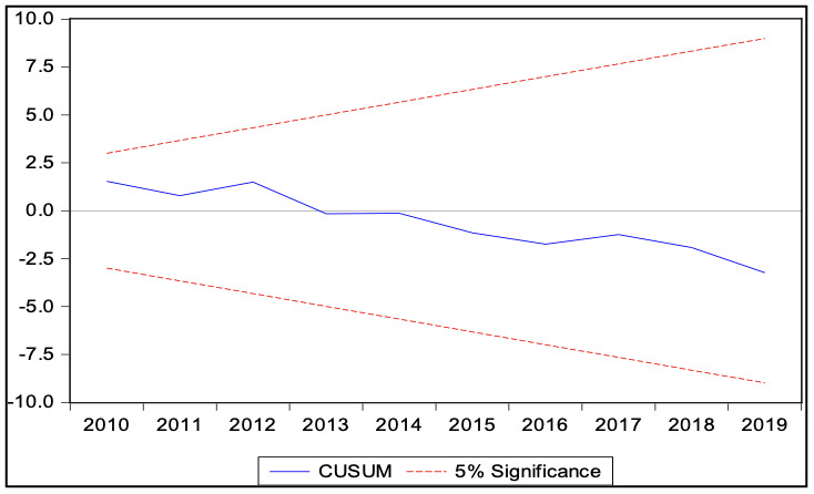
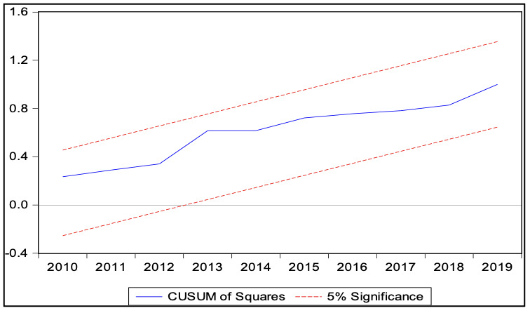
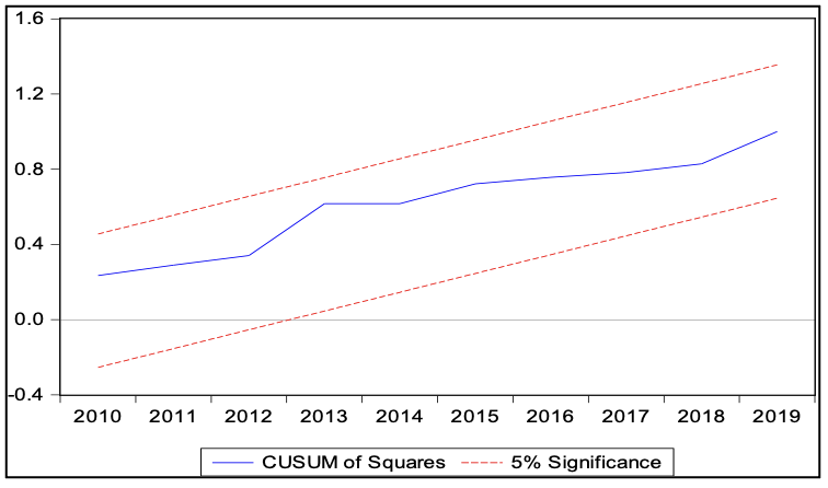
Furthermore, the diagnostic test results presented in Table 4 indicate normality of residuals, absence of serial correlation, and lack of heteroskedasticity issues within the model specifications. Additionally, the CUSUM and CUSUMQ tests detailed in the appendix confirm the model’s stability. Collectively, these findings point to an optimal fit for the empirical specification.
IV. Conclusion
This study investigates the energy requirements for enhancing farm productivity in Indian agriculture by analyzing the impact of power sector investment (rural electrification) and power subsidies on agricultural productivity (TFP) in India. The ARDL model results indicate that rural electrification improves farm TFP both in the short and long term. However, power subsidies do not significantly influence TFP in the short term and have a negative impact in the long term. Private farm investments and various forms of public investment are also significant determinants of farm TFP.
The policy recommendation of the study advocates for a shift from a subsidy-oriented approach to an investment-focused strategy that emphasizes the development of productive infrastructure in rural areas and the expansion of electrification in underserved or unelectrified villages. This is because power subsidies entail substantial environmental and economic costs and are unevenly distributed across states and among different farming groups.
Acknowledgement
The authors are grateful to two anonymous reviewers for their helpful suggestions. However, the usual disclaimer applies.