
I. Introduction
Crude oil pricing and its relationship with potential bubbles have become central issues in economic research. Floros and Galyfianakis (2020) define a bubble as a high level of trading volume in a particular asset class at prices well above its intrinsic value. Bubbles in energy prices are undoubtedly among the most serious threats to the stability of equity markets and global economic indicators. Over the past two decades, researchers have increasingly focused on identifying the main causes and consequences of bubbles in the energy market (Floros & Galyfianakis, 2020; Liu & Lee, 2018).
Sornette, Woodard, and Zhou (2009), along with Wu and Zhang (2014), demonstrated that bubble components exist within the behavior of energy prices. In line with this, other authors have noted that the timing of bubbles often coincides with specific events in financial markets, such as financial crises and geopolitical tensions, including wars (Fantazzini, 2016; Sornette et al., 2009; Su et al., 2017). Studies reveal a strong causal relationship and dynamic co-movement between oil prices and geopolitical concerns, particularly in the short term (Li et al., 2020). Trends in geopolitical risks have been shown to predict both in-sample and out-of-sample oil prices, providing relevant information beyond financial and commodity fundamentals (Zhang et al., 2022).
In many countries, a bidirectional causal relationship has been found between geopolitical risk and oil price trends, with a few exceptions showing a unidirectional relationship (Shahbaz et al., 2024). Furthermore, supply, demand, inventories, speculation, and international economic activity serve as key transmission mechanisms through which geopolitical issues indirectly impact oil prices (Lee et al., 2021; Olasehinde-Williams et al., 2023). The short- to medium-term effects of geopolitical threats on oil markets have become increasingly evident, with economic activity and speculation potentially exerting divergent influences on oil prices (Jiao et al., 2023).
With the onset of the Russian-Ukrainian war and the Middle East conflict, many energy analysts concluded that the continuation of the war has greatly contributed to the rise in oil prices. This is most evident in the increase of Brent crude oil prices from $101.29 on February 24, 2022 (the first day of the war), to $133.18 on March 8, 2022 (the ninth day of the war). At the same time, punitive measures were imposed on Moscow. These sanctions included preventing Russia from using the SWIFT system to transfer funds, freezing the assets of Russian banks in some countries, suspending export licenses for goods that can be used for civilian and military purposes, halting the export of high-tech goods and oil refining equipment, and setting limits on the amounts of money that Russians can deposit in banks.
As a result, global markets continue to bear the cost, with expectations of price bubbles and new records amid high global inflation and stagnation. Moreover, as oil is the world’s most commonly traded commodity and a major economic variable, movements in Brent and WTI prices have significant implications for the global economy and financial markets. Therefore, it is crucial to analyze their co-explosivity.
The primary goal of this study is to determine whether market speculation or geopolitical instability contributes more to oil price volatility. While previous research has explored the impact of geopolitical risks and financial speculation on oil markets, the findings remain inconclusive, with studies often focusing on isolated events or specific market conditions. Additionally, existing literature lacks a comprehensive analysis that compares the relative influence of these two factors during prolonged geopolitical conflicts, such as the Ukraine-Russia war. By addressing these gaps, this study aims to provide a clearer understanding of the key drivers of oil price fluctuations, helping investors and policymakers develop more effective risk management strategies.
The remainder of this paper is structured as follows: Section II presents the data and methodology, Section III discusses the empirical results, and Section IV concludes.
II. Data and Methodology
In this study, we use daily crude oil price data measured in U.S. dollars per barrel of oil, collected from the U.S. Energy Information Administration. The dataset includes Crude Oil Prices: West Texas Intermediate (WTI), Europe Brent Spot Price, and the geopolitical risk index (Caldara & Iacoviello, 2022). The period spans from 01 February 2020 to 11 December 2024, with observations recorded daily.
To examine bubble activity in oil prices, we employ the recent bubble detection procedures—the supremum ADF (SADF) test proposed by Phillips, Wu, and Yu (2011), and the generalized SADF (GSADF) test developed by Phillips, Shi, and Yu (2015). The supremum ADF test involves obtaining subsamples from the dataset and performing the Dickey-Fuller test on each subsample. The subsamples are defined as fractions of the entire dataset, denoted as where represents the complete dataset and The sample size increases iteratively, starting from the smallest possible size, denoted as up to the full dataset. The ADF test is applied at each iteration.
For each subsample, an autoregressive series is specified as follows:
Δyt=αr1,r2+λr1,r2yt−1+q∑j=1θqj1,r2Δyt−j
where represents oil price, and are parameters estimated using OLS. The subscripts and denote fractions of the total sample size T that specify the starting and ending points of a sub-sample period. q represents the number of lags which is set according to Bayesian Information Criterion. The null hypothesis is : against alternative explosive bubbles is : For each new regression, the sub-sample is created by merging the sub-sample from the preceding iteration with new observations. Assuming each sub-sample has a size denoted as , the coefficient test statistic and the Dickey-Fuller statistic are as follows:
DFλr=τ(ˆλτ(τ)−1),DFtτ=(∑τj=1y−j−1ˆστ)12(ˆλτ(τ)−1)
where represents the least squares estimate of which is based on the first observations denotes estimated value of and values are then compared with the critical values of the DF test.
The SADF statistics is:
SADF(r0)=supr2∈[r0,1]ADFr20
However, Phillips, Shi, and Yu (2015) contend that the SADF test is ineffective when multiple bubbles exist within the data. To address this limitation, they introduce an alternative method known as the GSADF test. This approach utilizes the Dickey-Fuller test across a series of subsamples from the dataset, adjusting both the end points and start points of each subset. The GSADF statistic is defined as follows:
GSADF(r0)=supr2∈[r0,1],r1∈[0,r2−r0]ADFr2r1
Following the detection of explosive behavior using the GSADF test, the start and end dates of bubble periods can be identified through backward SADF (BSADF) as outlined in Phillips, Shi, and Yu (2015):
BSADFr2(r0)=supr1∈[0,r2−r0]SADFr2r1
where the end of the rolling interval window is fixed at and the window size expands from to . Explosiveness periods are defined using the GSADF test as follows:
ˆre=infr2∈[r0,1]{r2:BSADFr2(r0)>scuαr2}
and
ˆrf=infr2∈[ˆre,1]{r2:BSADFr2(r0)<scuαr2}
where is the critical value of the SADF test for the observations. Following Harvey, Leybourne, and Sollis (2017), we use wild bootstrapping to address non-stationary volatility. Simulations are based on 5,000 replications.
To investigate the co-explosivity of oil prices, we will use the method described in Bouri, Shahzad, and Roubaud (2019) and apply the following logistic regression:
log(P(Y=1∣X)1−P(Y=1∣X))=β0+βiXi,t+ϵl
where Y is a dummy variable for WTI that takes the value one if when there is price explosiveness and zero if is a constant and represents dummy variable for Brent constructed in a similar way to Y.
Logistic regression, unlike linear regression, does not assume a normal distribution of predictors. This is advantageous since oil prices frequently exhibit skewed or non-normal distributions. Moreover, the logistic function generates probabilities ranging from 0 to 1, enabling the evaluation of the likelihood of co-explosivity between WTI and Brent. This function is essential for determining the extent of the relationship between potential influencing factors and co-explosivity.
III. Empirical Results
The results of SADF and GSADF tests are presented in Table 1 and Figure 1. The findings indicate that both SADF and GSADF tests are statistically significant at the 1% and 5% levels. The dashed areas in Figure 1 represent the explosive periods in WTI and Brent. The first instance of explosivity experienced by WTI occurred from 25 February 2021 to 26 February 2021, while for Brent, it occurred from 23 February 2021 to 01 March 2021. The price of a barrel of oil has risen sharply since the beginning of 2021, increasing from 50 dollars to 68 dollars per barrel—an increase of nearly 35%.
The primary explanation for the rise in oil prices is the strong economic recovery in China. Industrial production in China increased by almost 35% in January-February 2021 compared to the same period in 2020 (China, Statistics, 2021). This recovery is driving up the demand for oil, and consequently, its price. Additionally, the global economic recovery anticipated for 2021 by the World Bank, along with various stimulus plans, including the American plan totaling nearly 1.9 billion dollars, has contributed to further increases in oil prices during 2022.
Another factor in the rise in oil prices is the decision made in early March 2021 by the Organization of the Petroleum Exporting Countries (OPEC) and Russia to maintain the strict quota policy implemented one year prior. By voluntarily limiting the supply of oil, this quota policy mechanically exerts upward pressure on the price of crude oil.
Although the current price of oil remains well below its historical average of 109 dollars in 2013, this increase contrasts sharply with the evolution of the price of oil in 2020. When the COVID-19 pandemic erupted, the price of a barrel of oil fell drastically: from 67.8 dollars at the end of 2019 to only 15 dollars by early April 2020. This was due to the shutdown of some of the world’s major economies and the fall in air traffic. The WTI price of American oil even became temporarily negative due to near saturation of storage capacities.
Further instances of explosivity were observed during March 2022 within the Ukrainian-Russian conflict. Explosivity appeared first in Brent from 02 March 2022 to 04 March 2022 and in WTI from 04 March 2022 to 09 March 2022. With the escalation of the conflict in Ukraine and the almost total halt of Russian oil exports, the price of oil soared. This rise was caused by fears that the West would impose sanctions on Russian oil sales, as well as delays in finding a resolution to the Iran nuclear deal. Even though Western sanctions have not gone as far as banning Russian exports, the supply is affected, particularly because certain financial and banking sanctions make purchases from Russia difficult.
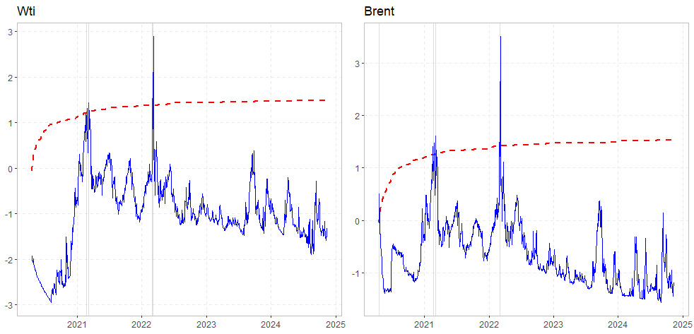
Table 2 shows that an increase in Brent crude prices raises the probability of higher WTI crude prices. This relationship is particularly evident during geopolitical events like the Russian-Ukrainian war, driven by fears of sanctions on Russian oil disrupting supply. Rising Brent prices due to geopolitical tensions directly affect US crude prices, irrespective of demand and supply. These findings align with studies by Ajmi, Hammoudeh, and Mokni (2021) and Khan et al. (2021).
However, there is no observed effect of geopolitical instability on WTI price explosiveness. WTI price dynamics are influenced more by domestic production and regional factors, making it less sensitive to global geopolitical events. Additionally, US energy independence and structural factors in the domestic oil market provide some protection against direct disruptions from geopolitical instability.
To check robustness, the relationship between geopolitical risk (GPR), WTI, and Brent at different quantiles was estimated using quantile regression. Table 3 shows that higher Brent prices positively affect WTI prices across all quantiles, while increased geopolitical risk negatively impacts WTI oil prices due to economic uncertainty lowering demand. Additionally, a stronger US dollar makes oil more expensive for foreign buyers, reducing demand further. Markets may anticipate rising production or strategic reserve releases, and speculative traders might sell oil short during expected global slowdowns. Geopolitical risks in major consuming regions can reduce industrial activity, leading to lower prices.
Geopolitical instability increases Brent crude prices by creating supply disruptions, market uncertainties, and transportation risks. Conflicts or sanctions in major oil-producing areas reduce supply, while threats to key routes like the Strait of Hormuz raise transport costs. Investors add a risk premium, causing speculative buying and price hikes. Stockpiling oil for potential shortages boosts demand, and currency fluctuations, especially a weaker US dollar, make oil pricier for global buyers, driving Brent prices higher.
IV. Conclusion
This study applies the SADF and GSADF tests (Phillips et al., 2011, 2015) to identify the beginning and end of potential speculative bubbles in the crude oil market during the Ukraine-Russia war. Results revealed evidence of multiple periods of bubble explosivity from 02 March to 04 March 2022. Moreover, findings indicate that the likelihood of explosiveness in WTI depends on the presence of explosiveness in the Brent price. The outcomes of this study are notable for at least one key reason: a bubble in the oil market may signal economic concern among investors, which could serve as an early indicator of a financial crisis, prompting policymakers to develop effective financial strategies.
The findings of this study offer several policy recommendations. Policymakers should consider enhancing market transparency, regulating speculative trading, and adjusting monetary policy to manage inflationary pressures stemming from energy price fluctuations. Additionally, improving geopolitical risk assessments, promoting energy diversification, and encouraging the development of hedging mechanisms can mitigate the economic impact of oil price shocks. Overall, these strategies will contribute to stabilizing markets and reducing vulnerabilities to future geopolitical tensions and energy price bubbles.