The Effect of Oil Price Uncertainty on the Joint Default Risk of Oil and Natural Gas Companies

I. Introduction

The U.S. oil and gas upstream sector has experienced significant transformation due to the growth of shale production. As of 2023, the United States produces over 13 million barrels of oil daily (accounting for 15% of global output) and 20% of the world’s natural gas, with 40% coming from shale extraction. Shale extraction requires substantial capital investment, causing firms to rely heavily on debt financing. By 2020, North American oil and gas companies held $86 billion in debt, which increased their financial vulnerability due to lower credit ratings compared to other industries.

In the global oil market, oil and gas companies act as price takers, making them highly susceptible to price volatility. Existing research indicates that oil price volatility adversely affects profitability (e.g., Song & Yang, 2022), disrupts cash flow (e.g., Maghyereh & Abdoh, 2020), and exacerbates financial distress in highly leveraged firms. Moreover, heightened volatility raises capital costs due to increased systematic risk premiums (Bali & Zhou, 2012), thereby amplifying the likelihood of default.

Systemic default risk within the oil and gas sector arises from the interconnectedness of firms. The sector’s oligopolistic structure, shared technologies, regulatory environment, and supply chain integration heighten the potential for contagion effects during periods of volatility. This interconnectedness, combined with significant government oversight due to the strategic importance of oil production, increases the risk of simultaneous defaults across multiple firms (Lee & Lee, 2019). Despite the well-documented relationship between oil price dynamics and macroeconomic outcomes (e.g., Amin et al., 2023; Elder & Serletis, 2010; Serletis & Xu, 2018), the role of oil price uncertainty (OPU) in predicting systemic default risk remains underexplored.

Our study addresses this gap by investigating the predictive power of OPU in forecasting systemic default risk for U.S. oil and gas firms. Previous studies have concentrated on the macroeconomic and firm-level consequences of oil price volatility (e.g., Kilian & Park, 2009). However, limited attention has been given to the systemic implications of oil price uncertainty within the energy sector. By applying the conditional prediction of the joint probability of default (CoJPoD) framework developed by Radev (2022), based on Segoviano & Goodhart’s (2009) minimum cross-entropy approach, we provide new insights into how OPU influences systemic risk dynamics. This method captures contagion and market sentiment effects via CDS spreads, offering a robust measure of systemic risk.

Our in-sample and out-of-sample analyses demonstrate that oil price uncertainty (OPU) significantly improves joint probability of default (JPoD) predictions, even after controlling for macroeconomic variables. Implied volatility measures outperform realized volatility in capturing systemic risk dynamics, aligning with prior studies (e.g., Bollerslev et al., 2009; Poon & Granger, 2003). By integrating OPU into systemic risk models, we highlight the importance of oil price dynamics for more accurate financial risk forecasts, particularly over longer horizons.

II. Methodology

Following Radev (2022), we consider a system with logarithmic returns $X_{1},\ X_{2},\ldots,X_{n}$ represented by random variables $x_1$, $x_{2}$, $\ldots$, $x_{n}$ in $n$, identifying the default region in the upper tail of the return distribution. The JPoD at time $t$ takes the following form:

$$\scriptsize{\begin{aligned} & {JPoD}_{t}(x_{1},\ x_{2},\ldots,x_{n})\\ & = \int_{{\overline{x}}_{1}}^{+ \infty}{\int_{{\overline{x}}_{2}}^{+ \infty}{\ldots\int_{{\overline{x}}_{n}}^{+ \infty}{p_{t + 1}(}}}x_{1},\ x_{2},\ldots,x_{n})dx_{1},\ {dx}_{2},\ldots,{dx}_{n}, \end{aligned}}\tag{1}$$

where $p_{t + 1}{(x}_{1},\ x_{2},\ldots,x_{n})$ is the time-varying conditional joint probability density, and ${\overline{x}}_{1},\ {\overline{x}}_{2},\ldots,{\overline{x}}_{n}$ are fixed default thresholds estimated using the CIMDO copula method.

A joint default occurs when n firms fall below their default thresholds. CoJPoD conditional on firm k, is defined as:

$$\small{\begin{aligned} & Co{JPoD}_{t}(system)\\ &= {JPoD}_{t}\left( x_{1},\ x_{2},\ldots,x_{k - 1},x_{k + 1},\ldots,x_{n}\left| x_{k} > {\overline{x}}_{k} \right. \right)\\ & = \frac{{JPoD}_{t}(system)}{{PoD}_{t}^{k}} \end{aligned}}\tag{2}$$

where ${PoD}_{t}^{k}$ is k’s default probability estimated via bootstrapping using five-year CDS spreads (${CDS}_{t}$):

$${PoD}_{t + 1}^{k} = \frac{{CDS}_{t} \times 0.0001}{1 - RR}\tag{3}$$

where $RR$ represents the recovery rate, typically assumed at 40% in academic and practical contexts (Radev, 2022).

Our primary objective is to determine if OPU can predict systemic defaults among energy companies, serving as an early warning tool. We begin with the following in-sample single-factor predictive model:

$${CoJPoD}_{t} = \alpha + \beta{OPU}_{t - 1} + \varepsilon_{t},\tag{4}$$

where OPU is a measure of oil price uncertainty, and $\varepsilon_{t}$ is a zero-mean disturbance term. The in-sample test assumes $\beta$ = 0 for no $OPU$ predictive power. However, OLS is unsuitable for high-frequency data due to conditional heteroscedasticity, persistence, and endogeneity, which complicate estimation. Alternative methods are needed to address these challenges and ensure accurate model evaluation (e.g., Salisu et al., 2019). To account for these features, Westerlund & Narayan (2015) suggested redefining Equation (4) as follows:

$${CoJPoD}_{t} = \delta + \beta{OPU}_{t - 1} + \gamma\left( {OPU}_{t} - \sigma{OPU}_{t - 1} \right).\tag{5}$$

In this equation, $\delta = \alpha - \gamma\theta$, where $\theta$ is the intercept of the AR(1) process: ${CoJPoD}_{t} = \theta + {\rho\ CoJPoD}_{t - 1}$. To reduce bias, the bias-adjusted OLS estimate of $\beta$ is as follows:

$${\widehat{\beta}}_{adj} = \widehat{\beta} - \gamma\left( \widehat{\rho} - \rho \right)\tag{6}$$

When there is no persistence and endogeneity effects, $\widehat{\beta} = {\widehat{\beta}}_{adj}$ in the sense that $\gamma\left( {OPU}_{t} - \sigma{OPU}_{t - 1} \right) = 0.$ To address conditional heteroscedasticity, we use a feasible quasi-generalized least squares estimator (Westerlund & Narayan, 2015), assuming ARCH process errors.

We then expand the analysis by adding predictors for macroeconomic conditions, including the economic policy uncertainty index (EPU), the Aruoba–Diebold–Scotti business conditions index (ADS), and the effective federal funds rate (FFR). We use the following predictive equation:

$${CoJPoD}_{t} = \alpha + \beta{OPU}_{t - 1} + \vartheta^{\mathstrut'}X_{i,t - 1}{+ \varepsilon}_{t,}\tag{7}$$

where $X_{i,t}$ is a set of predictors that capture macroeconomic conditions. The null hypothesis ϑ = 0 signifies no predictability in the relevant predictors. To assess forecasting precision, we used four loss functions: root mean squared error (RMSE), mean absolute error (MAE), mean percentage error (MPE), and mean absolute percentage error (MAPE). Lower values in these metrics indicate more accurate forecasts.

To evaluate OPU’s out-of-sample predictability, we split the dataset: the first block (January 3, 2004–January 15, 2019) estimated model parameters (75% of data), and the second (January 16, 2019–January 19, 2024) served as the forecasting period (25%). We employed the Diebold-Mariano (DM) test, a robust and widely accepted method for comparing forecast accuracy in out-of-sample evaluations. While the DM test has limitations in the context of nested models, this concern is not applicable here, as the models being compared—including the benchmark pure autoregressive model—are non-nested. Furthermore, the inclusion of additional performance metrics—MAPE, RMSE, MAE, and CPE—provides a comprehensive assessment of forecast performance, ensuring a more well-rounded and reliable analysis.^[1]

III. Sample and Data

This study calculates the CoJPoD for 21 US-listed oil and gas companies with 5-year CDS data from January 3, 2004, to January 19, 2024. Using Radev (2022) methodology, we employ 5-year US Treasury yields for refinancing rates and generate daily default probabilities from CDS spreads and bond yields from Bloomberg.

We analyze three OPU measures: (1) OPU-GARCH from Elder & Serletis (2010), (2) OPU-SV from a single-variable SV model, and (3) OPU-OVX from the CBOE Crude Oil ETF Volatility Index. Daily U.S. refiners’ crude oil acquisition costs (EIA) are used in GARCH and SV models, while OVX, EPU, ADS, and FFR data come from Thomson Reuters’ Datastream. Descriptive statistics of these variables are in Table 1.

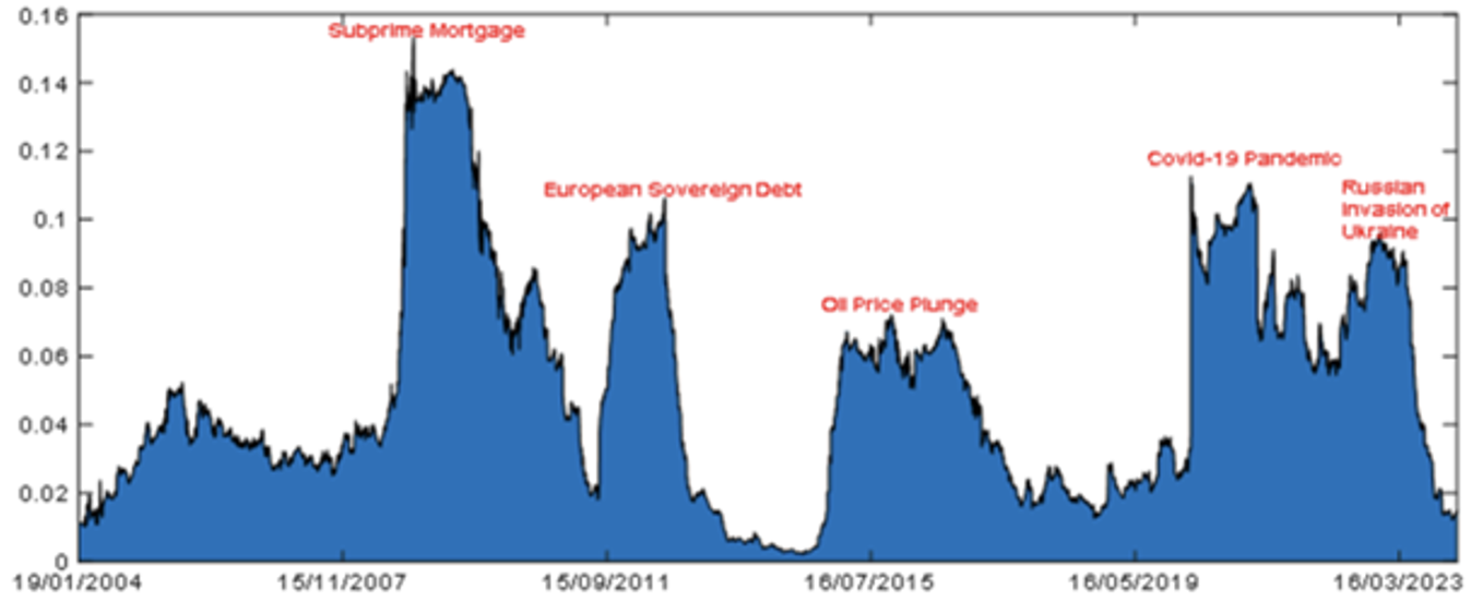
Figure 1 shows CoJPoD trends from January 3, 2004, to January 19, 2024. It began at a low level, increased during the Global Financial Crisis, then decreased until the Eurozone crisis in 2011 and the oil price crash in 2016. The COVID-19 crisis and subsequent geopolitical and economic factors led to an increase in systemic default risk.

Figure 1.The estimated value of CoJPoD

This figure presents the estimated values of the conditional joint probability of default (CoJPoD) over time, capturing joint default risk of oil and natural gas companies dynamics. The shaded blue area represents the CoJPoD, which measures the likelihood that multiple entities will default simultaneously under stressed conditions. The x-axis denotes the timeline from January 3, 2004, to January 19, 2024, while the y-axis represents the estimated probability values.

IV. Empirical Results

Our main hypothesis posits that OPU measures serve as indicators for future JPoD risk. Table 2 (Panel A) shows all OPU measures are positively significant in single-factor models (columns 1–3) and remain significant in multiple-factor models (columns 4–6), confirming OPU’s predictive accuracy for systemic default risk. Adjusted R² exceeds 19%, with OPU-OVX (implied volatility) outperforming OPU-GARCH and OPU-SV (realized volatility). Control variables enhance R², improving systemic risk prediction. Implied OPU, derived from options prices, reflects market expectations and sentiments about future oil price movements, capturing events not in historical data. Panel B shows loss functions (RMSE, MAE, MPE, MAPE) for in-sample forecasts, confirming OPU-OVX (implied volatility) offers the best accuracy in predicting systemic default risk.

Table 3 (Panel A) presents out-of-sample results that compare six predictive models to a pure autoregressive framework using four loss functions and DM statistics. The results indicate that OPU indicators significantly enhance the accuracy of predicting systemic default risk. Measures of implied volatility outperform those of realized volatility, exhibiting lower loss function values and higher DM statistics, which reflect stronger predictive power. Additionally, the inclusion of control variables further improves prediction accuracy.

V. Conclusion

This study explores the predictive capability of oil price uncertainty (OPU) for the joint probability of default (JPoD) among U.S. oil and gas companies. Through in- and out-of-sample analyses, it is observed that OPU significantly improves JPoD forecasts, even when accounting for macroeconomic factors. Implied volatility measures (e.g., OPU-OVX) are found to outperform realized volatility (e.g., OPU-GARCH, OPU-SV), indicating their superior capacity to capture systemic risk dynamics. These results highlight OPU’s important role in enhancing systemic default risk predictions, particularly over longer periods.

The findings provide practical insights for energy companies, regulators, and investors. Companies can incorporate OPU into risk management frameworks to identify vulnerabilities and adjust hedging or financing strategies. Regulators can utilize OPU to monitor systemic risks and implement timely interventions, such as stress tests or targeted safeguards. Investors can use OPU for improved risk assessment and portfolio allocation in volatile markets.

Future research could examine integrating OPU with other uncertainty measures or extending its application to sectors exposed to commodity price volatility. Improving systemic risk forecasting models will contribute to a more resilient and sustainable financial market.

Funding

This work was supported by the United Arab Emirates University [College Annual Research Program (CARP)-Spring 2024].