I. Introduction
The COVID-19 pandemic significantly impacted oil prices, creating disruptions on both supply and demand sides (Padhan & Prabheesh, 2021), which resulted in increased volatility in oil prices, particularly from 2020 onward (Ertuğrul et al., 2020).
Additionally, market efficiency, such as that of WTI oil prices, changed notably during the pandemic, shifting from efficiency to inefficiency as the price data from this period were analyzed (Gil-Alana & Monge, 2020). Price fluctuations in this market have broad economic implications, especially during times of global instability.
The primary motivation for studying this topic stems from the gasoline market’s role in a country’s economy, directly influencing consumers’ cost of living and businesses’ production costs and mobility (Barassi et al., 2022). Diesel and gasoline, as main petroleum-derived fuels, were significantly affected by the shocks of COVID-19 (Quintino & Ferreira, 2021), underscoring the importance of understanding their price dynamics.
The Russia-Ukraine war also considerably affected the main US energy markets, specifically oil, natural gas, and ethanol, leading to high price volatility and changes in the correlation strength between these markets post-outbreak (Quintino et al., 2023). This conflict disrupted global energy supply chains, increasing price fluctuations in the US gasoline market, which is crucial for economic stability.
Regarding the US gasoline market, there is limited literature on price persistence, with Gil-Alana and Payne (2017) being an exception. This reveals a gap: the recent dynamics of US gasoline prices, particularly in response to global shocks, remain underexplored. To address this gap, we analyze the persistence degree of US gasoline prices from January 1995 to December 2023, covering the recent impacts of the COVID-19 pandemic and the Russia-Ukraine war. We use detrended fluctuation analysis (DFA) with sliding windows to estimate the Hurst Exponent (H), a common measure of long-range dependence.
This study contributes to the literature in three ways: i) by examining the recent dynamics of gasoline prices, an essential economic asset affecting both consumers and companies; ii) by applying robust non-linear methods and sliding windows to capture the impacts of adverse shocks such as COVID-19 and the Russia-Ukraine conflict on their behavior; iii) by differentiating among gasoline types, it provides insights into the specific characteristics of each.
II. Methodology and Data
We utilize weekly US gasoline prices, specifically Regular Conventional (RC), Midgrade Conventional (MC), Premium Conventional (PC), and All Grades Conventional (AGC), spanning from January 2, 1995, to December 25, 2023. The data can be accessed publicly via the US Energy Information Association (U.S. E.I.A) at https://www.eia.gov/petroleum/data.php#prices. This extensive period allows for a thorough assessment of long-term trends and persistence in gasoline prices, enabling the capture of significant economic, political, and social events that could influence gasoline price behavior.
Notably, this period includes recent major events such as the COVID-19 pandemic and the Russian-Ukrainian conflict, which have had profound impacts on global energy markets. The pandemic led to demand shocks and supply chain disruptions, whereas the Russian-Ukrainian war has caused volatility in oil supply and prices due to sanctions and geopolitical instability.
By covering this comprehensive timeline, the study aims to evaluate how these extreme events affect the persistence of gasoline prices, offering relevant and timely insights into the current economic environment. Furthermore, beginning the analysis in 1995 allows consideration of the influences of globalization, technological advancements, and shifts in energy policies over time. This provides a contextually rich analysis that spans various phases of economic development and energy policy, rendering the findings applicable to diverse contexts.
The DFA approach proposed by Peng et al. (1994) allows the evaluation of long-range dependence in financial time series even when data is nonstationary, overcoming these limitations [see Peng et al. (1995) for the complete DFA procedure]. The final step of this procedure involves analyzing the behavior of the fluctuation function which follows a power law of 𝑛, i.e., and is characterized as the long-range autocorrelation exponent of the DFA method. This exponent represents the the memory effect of the series and quantifies the empirical strength of the long-range power-law autocorrelation. It is also used to identify the level of persistence (Zebende et al., 2017).
If there exists no long-range autocorrelation in the series (no memory), the series could be described as a random walk. On the other, if the series has long-range anti-persistent (negative) autocorrelation, and if the series has long-range persistent (positive) autocorrelation.
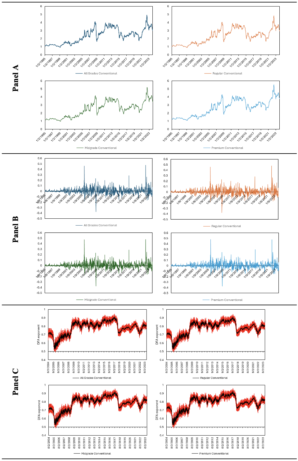
To analyze the dynamic behaviour of the exponent and overcome the limitation of arbitrarily dividing data into subsamples, we applied the sliding windows approach. The window lengths must be sufficiently large to ensure statistical significance while remaining small enough to retain sensitivity to change scaling properties over time (Morales et al., 2012). Based on our sample size and following Matcharashvili et al. (2016), we utilized windows of 500 observations. As illustrated in Figure 1 (Panel C), we estimated all the exponents for the first differences in US gasoline prices.
III. Results
Table 1 presents the primary descriptive statistics for US gasoline prices. AGC and RC gasoline prices approached $5 per gallon, whereas MC and PC prices surpassed $5 per gallon. Concerning the minimum values, all gasoline prices fell below $1 per gallon during the analyzed period, except for PC gasoline prices. The data exhibit slight positive skewness, indicating that the distributions of gasoline prices are moderately right-skewed, as confirmed by the Shapiro-Wilk test. Consequently, there is a minor tendency for higher prices to occur less frequently, albeit this effect is weak. In practical terms, most prices cluster around the mean, with a few higher outliers extending the distribution’s tail to the right. The kurtosis values are all below 3 (the kurtosis of a normal distribution), suggesting platykurtic distributions. This implies thinner tails than a normal distribution, with fewer extreme values, indicating that gasoline prices are less susceptible to extreme fluctuations and exhibit lower volatility, with fewer sharp spikes or drops.
Panel B of Figure 1 illustrates the first differences, showing consistent patterns across all types of US gasoline, with an increase in variance particularly noticeable after 2000. Notable peaks occurred in 2005, 2017, and 2022 (around the onset of the Russia-Ukraine conflict). These series exhibit a stationary pattern, which was corroborated by the Augmented Dickey-Fuller test results (-10.5995 for AGC, -10.6149 for RC, -10.5456 for MC, and -10.5883 for PC, all statistically significant at the 1% level). The test results enabled us to reject the null hypothesis, confirming that the series are stationary. This indicates that shocks to gasoline prices in their first-differenced form are likely transitory and do not have persistent effects.
However, it is important to note that the ADF test does not account for fractional integration or potential long-range dependencies within the series, due to its limited power against fractional unit roots (Diebold & Inoue, 2001; Hassler & Wolters, 1994).
The DFA approach proposed by Peng et al. (1994) was applied using sliding windows to address this limitation, evaluate the long-range dependence, and detect dynamic correlations. The results are shown in Figure 1, Panel C. All US gasoline prices exhibit a similar pattern, with indicating persistent behavior (the series has long-range positive autocorrelation). This implies that price fluctuations tend to be followed by similar movements in the same direction, resulting in a persistent effect over time. The persistence indicates that even though the first differences of the series are stationary, they still show a tendency for long-term memory or autocorrelation. Therefore, price movements are more likely to maintain a consistent direction over time rather than quickly reverting to the mean. In other words, mean reversion (where prices tend to return to a central long-term value after deviations) is less likely in this context.
Although the US gasoline types display the values vary slightly across the different gasoline types. For instance, PC tends to exhibit a slightly more persistent behavior than the other US gasoline types, with higher exponents in certain periods, indicating a greater resistance to sudden changes. Additionally, differences in short-term fluctuations can be identified, with small variations in the exponent over time appearing more pronounced in some gasoline types, such as MC and PC, which show more marked variations, while AGC and RC maintain more stable variations.
Analyzing the time evolution of the exponents, at the beginning of the analyzed period, the exponents of all the US gasoline types reveal a relatively moderate behavior, suggesting a more stable market with less persistence in price movements. This period coincides with a phase of economic stability before the major shocks that would occur in the following years. After the second half of 2005, all the US gasoline types show an increase in exponents, indicating an increase in long-term persistence. This behavior can be associated with the increase in oil prices and the global supply crisis during this period, largely influenced by geopolitical issues such as the Iraq War and the growing demand for oil in emerging economies such as China and India. During the period of the global financial crisis (2008-2010), the exponents registered again an increase and significant fluctuations.
The global economic collapse not only affected energy demand but also generated volatility in the markets, which justifies the strong persistence in gasoline price changes. During the COVID-19 pandemic, there was also an increase in persistence, a behavior that can be explained by mobility restrictions, disruptions in global supply chains, and a collapse in fuel demand, resulting in significant fluctuations in gasoline prices. Near the beginning of the war between Russia and Ukraine (in 2022), another significant increase in the exponents is observed (a high level of persistence). This armed conflict generated uncertainty in the global energy market, especially due to the Russian oil and gas sanctions, which impacted major global exporters.
__first_differences_of_us_gasoline_prices.png)
IV. Conclusion
The findings revealed that across all types of gasoline implies that price shocks have persistent effects. This means gasoline prices do not revert quickly to their long-term trend after shocks, such as those caused by the COVID-19 pandemic or the Russia-Ukraine war. The positive autocorrelation captured by exponents reflects a tendency for price movements to follow sustained increases or decreases rather than random fluctuations. From an economic policy perspective, this highlights the need for long-term strategies to stabilize the market and mitigate lasting impacts of shocks. Thus, managing price volatility effectively may require sustained interventions over time.
The persistence observed in all gasoline types revealed long-range persistence, responding similarly to major global events like the 2008 Financial Crisis, the COVID-19 pandemic, and the Russia-Ukraine war. The differences between US gasoline types are more evident in terms of response magnitude, with PC and MC showing more marked fluctuations.