I. Introduction
The issue of energy (in)security gained renewed attention in the 1970s, when several developed economies were impacted by shifting geopolitical dynamics. Energy insecurity encompasses various consequences arising from the unavailability of energy resources (Taghizadeh-Hesary et al., 2021). Increasing energy insecurity, driven by overreliance on the international energy market and energy price volatility, renders a country’s economic performance vulnerable. Wang et al. (2022) identified a negative impact of oil price volatility on economic growth in leading oil importer and exporter countries, while Banna et al. (2023) reported that heightened energy security risk diminishes economic growth for a panel of 68 countries. The utilization of renewable energy mitigates energy insecurity and simultaneously fosters economic growth (Hieu & Mai, 2023). Chu et al. (2023) demonstrated the inverse relationship between energy insecurity and renewable energy usage in the top 23 energy-consuming nations. Tugcu and Menegaki (2024) illustrated that renewable energy generation reduces energy security risks within G7 countries.
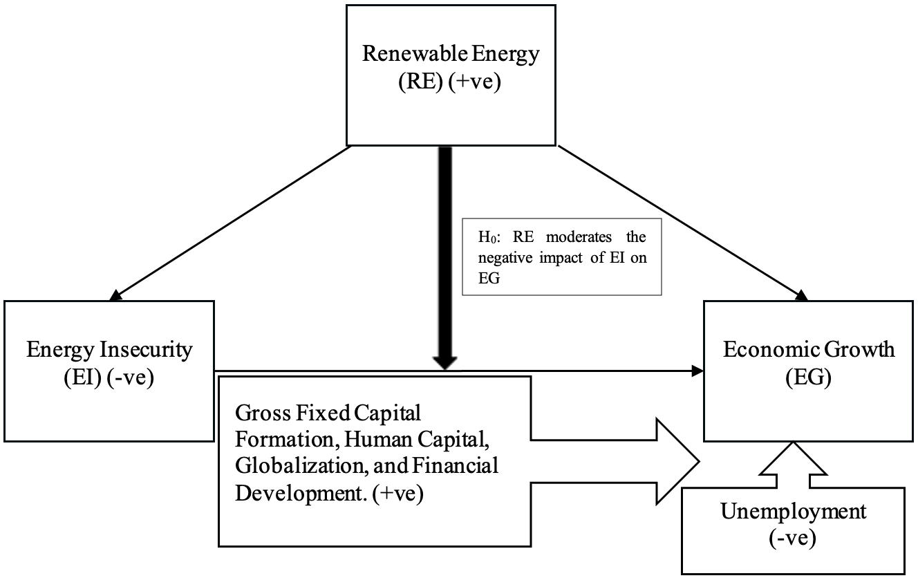
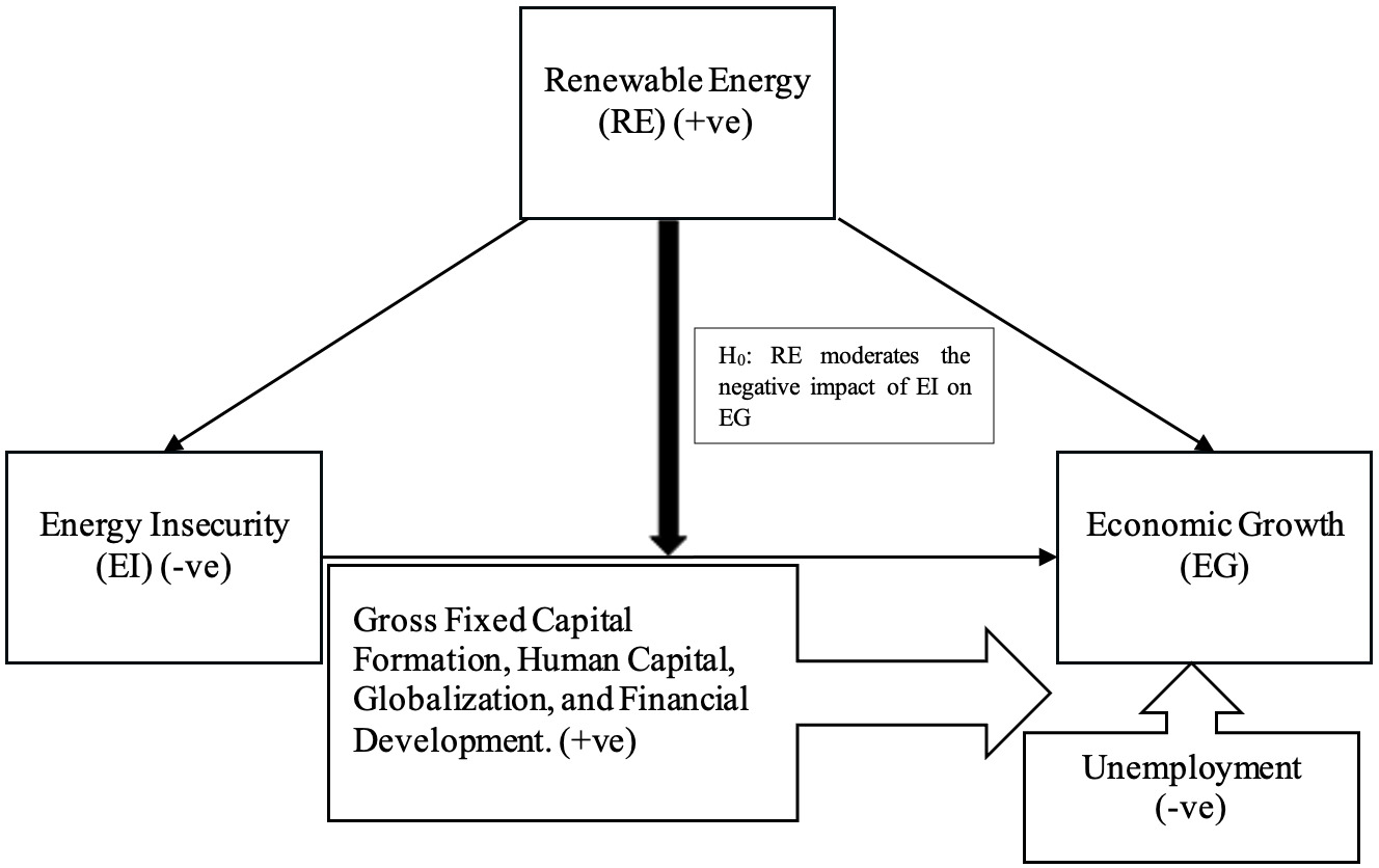
Given this context, it is reasonable to propose that renewable energy can counteract the negative effects of energy insecurity on economic growth, at least partially if not entirely. Nevertheless, few studies have examined this dynamic relationship among renewable energy, energy insecurity, and economic growth. This relationship has not been thoroughly investigated within the G20 framework, resulting in a research gap that the present study seeks to address. Besides energy, other factors also influence a country’s economic growth. For instance, Azam et al. (2023) highlighted the positive impact of gross fixed capital formation; Uddin and Rehman (2023) noted the adverse effect of unemployment; Khan et al. (2023) observed the beneficial effect of human capital; Sghaier (2023) revealed the positive influence of trade openness and financial development; and Sun et al. (2023) indicated the stimulating effect of globalization across different periods and locations. Thus, it is essential to control for these variables while examining the dynamic relationship among renewable energy, energy insecurity, and economic growth in net oil-importing G20 countries during 1990–2021, as outlined in the conceptual framework (Figure 1).
The G20 is a significant intergovernmental forum consisting of 19 sovereign countries, the European Union, and the African Union. It represents 85% of the world GDP, over 75% of global trade, and two-thirds of the global population (Government of India, 2024). The G20 consumes 80% of global energy, with 85% derived from non-renewable sources (Energy Institute, 2023). According to the International Renewable Energy Agency (IRENA), G20 countries have the potential to use 75% of the world’s renewable energy by 2030 (IRENA, 2018). Additionally, net oil-importing countries are more susceptible to risks in the global energy market. These factors make the net oil importers of the G20 ideal subjects for study.
The paper is structured as follows: Section II covers the data and methodology, Section III discusses the results, and the final section concludes the study.
II. Data and Methodology
A. Data
The study utilizes data from 27 net oil-importing G20 countries during the period of 1990–2021.[1] The five-year moving average method is employed to impute incomplete observations. The outcome variable of this study is economic growth, represented by per capita gross domestic product (PCGDP). The primary explanatory variable is energy insecurity, measured by the energy security risk index (ESR). Developed by the Global Energy Institute, this index captures a nation’s vulnerabilities to volatility in the energy market. The study incorporates two moderating variables: renewable energy consumption (REN) and the share of renewable energy in total energy consumption (RENS). Additionally, the study considers gross fixed capital formation (GFCF), unemployment (UMP), human capital (HC), globalization (GLO), and financial development (FD) as control variables (Table 1). All variables are transformed into natural logarithms for analysis.
Table 1 indicates that PCGDP exhibits the greatest variation (standard deviation = 15,830.070), whereas FD demonstrates the least variation (standard deviation = 0.211). This suggests that there are significant disparities in per capita income among the sample countries, while their financial situations are relatively similar. The J-B test statistic reveals that only PCGDP follows a normal distribution among all the variables.
B. Methodology
LnPCGDPit=α0+α1LnESRit+α2LnRENit+α3LnGFCFit+α4LnUMPt+α5LnHCit+α6LnGLOit+α7LnFDit+uit
LnPCGDPit=β0+β1LnESRit+β2LnRENSit+β3LnGFCFit+β4LnUMPt+β5LnHCit+β6LnGLOit+β7LnFDit+uit
Subscripts and represent cross-sections and time periods, respectively. Further, and are the intercepts, and represent the elasticity parameters to be estimated, and is the independent and identically (i.i.d) error term. To investigate the moderation impact of REN and RENS, an interaction term is included as follows:
LnPCGDPit=γ0+γ1LnESRit+γ2LnRENit+γ3(LnESRit×LnRENit)+γ4LnGFCFit+γ5LnUMPt+γ6LnHCit+γ7LnGLOit+γ8LnFDit+uit
LnPCGDPit=δ0+δ1LnESRit+δ2LnRENSit+δ3(LnESRit×LnRENSit)+δ4LnGFCFit+δ5LnUMPt+δ6LnHCit+δ7LnGLOit+δ8LnFDit+uit
The study uses the bias-adjusted Lagrange multiplier (LM) test (Pesaran et al., 2008) and the Pesaran cross-sectional dependence (CD) test (Pesaran, 2021) to check for cross-sectional dependence among panels. The findings indicate the presence of cross-sectional dependence, making second-generation methods appropriate for this analysis. To assess the stationarity of variables, the cross-sectionally augmented Im-Pesaran-Shin (CIPS) unit root test (Pesaran, 2007) is applied. Additionally, all diagnostic tests are conducted. Results from the Wooldridge and modified Wald tests reveal the existence of autocorrelation and heteroskedasticity, while the Hausman test supports the fixed effect model. Consequently, the fixed effect model with the Driscoll-Kraay standard error (DKSE) method (Driscoll & Kraay, 1998) and the feasible generalized least squares (FGLS) method (Parks, 1967) are employed. Moreover, as a non-parametric method, DKSE is robust when variables follow a non-normal distribution.
III. Main Findings
A. CD and CIPS tests
The findings from both CD tests strongly indicate the presence of cross-sectional dependence among the panels. Consequently, the CIPS unit root test was carried out, and the results demonstrate that ESR, REN, RENS, GLO, and FD are stationary at level [I(0)], while PCGDP, GFCF, UMP, and HC are stationary at first difference [I(1)] (see Table 2).
B. DKSE and FGLS methods
Table 3 indicates that the data are not poolable and exhibit issues with autocorrelation and heteroskedasticity. The average values of VIF for Models 1 and 2 are 1.84 and 1.83, respectively, which are below the threshold of 10[2], indicating no multicollinearity concerns. The Hausman test recommends the use of fixed effects in the models. Consequently, the fixed effect model with DKSE and FGLS methods is applied to assess the empirical relationships among the variables under consideration. Furthermore, Models 1 and 2 present results without moderation, while Models 3 and 4 demonstrate the moderating impact of REN and RENS, respectively.
Results indicate that ESR dampens economic growth in selected G20 nations, as risks and uncertainties in the global energy market disrupt the global supply chain, negatively affecting the countries’ economic performance. This finding aligns with the study by Banna et al. (2023). However, REN and RENS positively influence economic growth in these countries, consistent with Hieu and Mai’s (2023) findings. The coefficients of interaction terms are negative and smaller than the coefficient values of LnESR in the respective models. This suggests that while renewable energy usage moderates the adverse impact of energy insecurity on economic growth to some extent, it does not entirely offset the negative effects. Although the use of renewable energy has significantly increased in these economies, consumption levels have not yet reached a point where the threat of energy insecurity can be permanently eradicated. The marginal effect of ESR on PCGDP is -0.518 and -0.361, respectively. Additionally, GFCF, HC, GLO, and FD promote economic growth, whereas UMP hinders it in the selected economies.
IV. Conclusion
This study examines the moderating role of renewable energy on the relationship between energy insecurity and economic growth within G20 countries. The findings indicate that while energy insecurity negatively affects economic growth, renewable energy has a positive impact in certain G20 nations. Renewable energy is shown to partially mitigate the negative effects of energy insecurity on economic growth. Additionally, GFCF, HC, GLO, and FD are found to enhance economic growth, whereas UMP is found to hinder it.
Increasing the consumption of domestic renewable energy reduces a country’s dependence on the global energy market and its vulnerability to energy uncertainty. Therefore, it is recommended to promote the use of renewable energy in these economies. Furthermore, these countries should invest more in renewable energy plants and technologies to make renewable energy available at lower costs. They can also utilize digital platforms to raise awareness about renewable energy.
Australia, Austria, Belgium, Bulgaria, China, Croatia, Finland, France, Germany, Greece, Hungary, India, Indonesia, Ireland, Italy, Japan, Netherlands, Portugal, Romania, Slovak Republic, South Africa, South Korea, Spain, Sweden, Turkey, United Kingdom, United States. The African Union has been excluded from this study.
The result of VIF is available upon request.