Russia-Ukraine War and Oil Price: A TVP-VAR Analysis

I. Introduction

The theoretical framework of asset pricing is founded on two contrasting perspectives: the efficient market hypothesis and behavioural finance theory (Fakhry, 2016). According to the efficient market hypothesis, asset prices are determined by the available information. Conversely, behavioural finance theory suggests that asset prices are influenced by market participants’ reactions to this information. This dichotomy informs the ongoing debate regarding oil prices in the context of the Russia-Ukraine conflict, which has introduced new dynamics into international energy markets, including the oil market (Bassam et al., 2023).

The current geopolitical tension raises concerns about the stability of energy supplies from Russia, one of the largest crude oil producers in the world (Inacio et al., 2023). The ongoing conflict has the potential to create significant uncertainties that could severely impact the macroeconomy (Henzel & Rengel, 2017). In 2022, the oil market experienced a reduction in liquidity and open interest for both Brent and WTI, following the Russia-Ukraine conflict. This decline can be attributed to increased interest rates and the collateral requirements imposed by major exchanges.^[1] However, the dynamic interconnection between the Russia-Ukraine war and the global oil market is not thoroughly documented in the literature. Most previous studies have concentrated on the economy (Mbah & Wasum, 2022), international trade (Orhan, 2022), and financial markets (Umar et al., 2022). An exception is the study by Zhang et al. (2023) which explored the mechanisms through which the Russia-Ukraine war influences oil prices, employing the Complex Empirical Mode Decomposition (CEMD) method to predict high, medium, and low-frequency subsequences within a specific event window.

We thus examine the relationship between the Russia-Ukraine conflict and oil prices in several specific ways. First, we employ a comprehensive time-varying parameter vector autoregression (TVPVAR) model, as proposed by Antonakakis and Gabauer (2017). This approach significantly enhances the methodology established by Diebold and Yılmaz (2012) by eliminating the need for rolling-window methods and addressing issues related to outliers and unstable parameters, thereby improving the robustness of our analysis. Second, we address the findings of Sokhanvar & Lee (2023), which indicate that the euro exchange rate plays a significant role in the Russia-Ukraine conflict-oil price nexus, a point not explicitly examined in previous studies. This paper acknowledges and addresses this identified gap.

The remainder of the paper is organized as follows. Data and preliminary analysis are discussed in Section II; Section III analyzes the findings; and the paper concludes in Section IV.

II. Data and Methodology

The datasets utilized in this study are daily oil prices (WTI), US dollar/Euro exchange reference rates (EXH), and the Russian-Ukraine War Index (RUindex). The study period spans from February 24, 2022, to May 20, 2023. Data on WTI was obtained from investing.com, while the US dollar/Euro exchange rates were sourced from the European Central Bank (ECB). We employed the Russia-Ukraine War Index developed by Imandojemu & Sule (2024).

In this paper, we utilized the time-varying parameters vector autoregressive model (TVP-VAR) as proposed by Antonakakis and Gabauer (2017), which extends the connectedness model of Diebold and Yilmaz (2012). This model allows for the variance and covariance matrix to change over time. The basic TVP-VAR (p) model is formulated as follows:

$$y_{t} = A_{t}z_{t - 1} + \varepsilon_{t}\qquad\varepsilon_{t}\left| \Omega_{t - 1} \sim N\left( 0,\sum_{t} \right) \right.\tag{1}$$

$$vec\left( A_{t} \right) = vec\left( A_{t - 1} \right) + \varepsilon_{t}\qquad\varepsilon_{t}\left| \Omega_{t - 1} \sim N\left( 0,\Xi_{t} \right) \right.\tag{2}$$

With

$$z_{t - 1} = \begin{pmatrix} y_{t - 1} \\ y_{t - 2} \\ \vdots \\ y_{t - p} \end{pmatrix}A_{t}' = \begin{pmatrix} A_{1t} \\ A_{2t} \\ \cdots \\ A_{pt} \end{pmatrix} \tag{3}$$

where $\Sigma_{t}$ and $\Xi_{t}$ are the time-varying variance-covariance matrix with $m \times m$ and $m^{2}p \times m^{2}p$ dimension, $\Omega_{t - 1}$ captures all the information available till period $t - 1$. $Vec\left( A_{t} \right)$ is a vector of $\left( A_{t} \right)$ with $m^{2}p \times 1$ dimensions.

Thus, the Kalman multivariable filter is presented as follows:

$$\begin{aligned} & \operatorname{vec}\left(A_t\right) \mid z_{1: t-1} \quad \sim N\left(\operatorname{vec}\left(A_{t \mid-1}\right), \Sigma_{t \mid--1}^A\right) \\ & A_{t \mid t-1} \quad=\mathrm{A}_{t-1 \mid t-1} \\ & \epsilon_t \quad=y_t-\mathrm{A}_{t \mid \mathrm{t}-1} z_{1 \mathrm{t}-1} \\ & \Sigma_t \quad=\mathrm{k}_2 \Sigma_{\mathrm{t}-1 \mid \mathrm{t}-1}+\left(1-\mathrm{k}_2\right) \epsilon_t^{\prime} \epsilon_t \\ & \Xi_t \quad=\left(1-\mathrm{k}_1^{-1}\right) \Sigma_{\mathrm{t}-1 \mid \mathrm{t}-1}^A \\ & \Sigma_{t \mid t-1}^A \quad=\Sigma_{t-1 \mid t-1}^A+\Xi_t \\ & \Sigma_{t \mid t-1} \quad=\mathrm{z}_{t-1} \Sigma_{t \mid \mathrm{t}-1}^A \mathrm{z}_{\mathrm{t}-1}^{\prime}+\Sigma_t \end{aligned}$$

Hence, $A_{t},\Sigma_{f}^{A}$ is updated for time, t:

$$\begin{array}{l} {\text{vec}\left( A_{t} \right)\left| z_{\text{1:t}} \right. \sim N\left( \text{vec}\left( A_{t\left| t \right.} \right)\text{,}\text{Σ}_{t\left| t \right.}^{A} \right) }\\{K_{t} = \Sigma_{t\left| t - 1 \right.}^{A}z_{\text{t-1}}' \Sigma_{t\left| t - 1 \right.}^{- 1}}\\ {A_{t\left| t \right.} = \text{A}_{t\left| t - 1 \right.}\text{+}\text{K}_{t}\left( y_{t}\text{-}\text{A}_{t\left| \text{t-1} \right.}z_{\text{1t-1}} \right) }\\ {\Sigma_{t\left| t \right.}^{A} = \left( 1 - K_{t} \right)\Sigma_{t\left| \text{t-1} \right.}^{A}}\\ {\in_{t\left| t \right.} = \text{y}_{t} - A_{t\left| t \right.}z_{\text{t-1}} }\\ \Sigma_{t\left| t \right.} = \text{k}_{2}\Sigma_{\text{t-1}\left| \text{t-1} \right.} + \left( \text{1-}\text{k}_{2} \right)e_{t\left| t \right.}' e_{t\left| t \right.}\end{array}$$

$K_{t}$ is the Kalman gain that captures the dynamism of $A_{t}$ in any given state. The uncertainty parameter, $\Sigma_{t\left| \text{t-1} \right.}^{A}$, represents high (low) parameter which indicates how adjusted or similar it is to previous state, and $\Sigma_{t}$ indicates the error variance. Therefore, time-varying coefficient and variance-covariance matrices are used to compute the generalized connectedness of Diebold and Yilmaz (2014) using the generalized impulse response function (GIRF) and generalized forecast error variance decomposition (GFEVD). Thus, TVP-VAR is modified into a vector moving average based on the world representation theorem:

$$y_{t} = J' \left( M_{t}\left( z_{t - 1} + \eta_{t - 1} \right) + \eta_{t} \right) \tag{4}$$

$$y_{t} = J' \left( M_{t}\left( M_{t}\left( z_{t - 3} + \eta_{t - 2} \right) + \eta_{t - 1} \right) + \eta_{t} \right) \tag{5}$$

$$y_{t}\text{=}\text{J}' \left( M_{t}^{k - 1}z_{t - k - 1} + \sum_{j = 0}^{k}{M_{t}^{j}\eta_{t - j}} \right) \tag{6}$$

with

$$\small{M_{t} = \begin{pmatrix} A_{t} & \\ I_{m(p - 1)} & 0_{m(p - 1) \times m} \end{pmatrix}\eta_{t} = \begin{pmatrix} e_{t} \\ 0 \\ \vdots \\ 0 \end{pmatrix} = J \in_{t}J = \begin{pmatrix} 1 \\ 0 \\ \vdots \\ 0 \end{pmatrix}} \tag{7}$$

where $M_{t}$ is an $mp \times mp$ dimensional matrix, $\eta_{t}$ is an dimensional vector as $J$ is an $mp \times m$dimensional matrix. Taking limit as k approaches infinity $(\infty)$ yields to:

$$\begin{aligned} y_{t} &= \lim_{k \rightarrow \infty}J' \left( M_{t}^{k - 1}z_{t - k - 1} + \sum_{j = 0}^{k}{M_{t}^{j}\eta_{t - j}} \right)\\ & = \sum_{j = 0}^{\infty}{J' M_{t}^{j}\eta_{j - j,}} \end{aligned}\tag{8}$$

As it directly follows

$$y_{t} = \sum_{j = 0}^{\infty}{J' M_{i}^{j}J \in_{t - j}B_{jt} = J' M_{t}^{j}J,J} = 0,1,... \tag{9}$$

$$y_{t} = \sum_{j = 0}^{\infty}{B_{\text{jt}} \in_{\text{i-j}}} \tag{10}$$

where $B_{jt}$ is a matrix of $\times m$ dimensions.

The response of all J to a shock in variable I is given by GIRFs $\left( \psi_{ij,t}(H) \right)$ and since the model is non-structural, we employ H-step-ahead forecast model as follows:

$$\begin{aligned} GIRF_{t}\left( H,\delta_{j,t,}\Omega_{t - 1} \right) &= Ε\left( y_{t + H}\left| e_{j} = \delta_{j,t}\Omega_{t - 1} \right.\ \right)\\ & \quad - Ε\left( y_{i + 1}\left| \Omega_{t - 1} \right.\ \right) \end{aligned}\tag{11}$$

$$\psi_{j,t}(H) = \frac{B_{H,t}\Sigma_{t}e_{j}}{\sqrt{\Sigma_{jj,t}}} = \frac{\delta_{j,t}}{\sqrt{\Sigma_{jj,t}}}\delta_{j,t} = \sqrt{\Sigma_{jj,t}} \tag{12}$$

$$\psi_{j,t}(H) = \sum_{jj,t}^{- \frac{1}{2}}{B_{H,t}\Sigma_{t}e_{j}} \tag{13}$$

$e_{j}$ is a $m \times 1$ selection matrix with 1 on the j^th position and zero otherwise. The GFEVD which captures the directional pairwise connectedness from j to i is then computed as follows:

$${\bar{\phi}}_{ij,t}(H) = \frac{\sum_{i = 1}^{H - 1}\psi_{ij,t}^{2}}{\sum_{j = 1}^{w}{\sum_{i = 1}^{H - 1}\psi_{ij,t}^{2}}} \tag{14}$$

The numerator in Equation (14) reflects the overall impact of a shock in a specific variable $i$, while the denominator represents the combined effect of all shocks. The total connectedness can be calculated using the GFEVD as follows:

$$\begin{aligned} C_{i}(H) &= \frac{\sum_{i,j = 1,i \neq i}^{m}{{\bar{\phi}}_{ij,t}(H)}}{\sum_{i,j, = 1}^{11}{{\bar{\phi}}_{ij,t}(H)}}*100\\ &= \frac{\sum_{i,j = 1,i \neq j}^{m}{{\bar{\phi}}_{ij,t}(H)}}{m}\\ &= 100 \end{aligned}\tag{15}$$

Equation (15) shows the connectedness of the system. The directional connection to the system, indicating the shock impact that a variable $i$ transmits to the system of variables $j$ is computed as follows:

$$C_{i \rightarrow j,t}(H) = \frac{\sum_{j = 1,i \neq j}^{w}{{\bar{\phi}}_{ji,t}(H)}}{\sum_{i = 1}^{mi}{{\bar{\phi}}_{ji,t}(H)}}*100\tag{16}$$

Furthermore, the directional connection from the system, which demonstrates the impact of shocks received by a variable $i$ from the system of variables $j$, is defined as follows:

$$C_{i \leftarrow j,t}(H) = \frac{\sum_{j = 1,i \neq j}^{m}{\phi_{ij,t}(H)}}{\sum_{i = 1}^{mi}{\phi_{ij,t}(H)}}*100 \tag{17}$$

Thus, the net effect of the variable $i$ on the system—representing the difference between the impact transmitted to and received from the system—is determined as follows:

$$C_{i,t} = C_{i \rightarrow j,t}(H) - C_{i \leftarrow j,t}(H) \tag{18}$$

III. Empirical Analysis

Summary statistics for the variables of interest are presented in Table 1. The data indicates that the exchange rate has the lowest variance among the variables, followed by WTI and RUindex. This suggests that the exchange rate is the least volatile. Conversely, the RUindex shows the highest volatility, making it the riskiest variable. Furthermore, the analysis reveals that WTI and RUindex are significantly positively skewed, whereas the exchange rate is negatively skewed.

Notably, the kurtosis values of the variables of interest are less than three, indicating reduced market risk. The normality test performed by Jarque and Bera (1980) confirms that the RUindex is the only variable displaying a normal distribution. Furthermore, the ERS unit-root test results show that all series are non-stationary. According to the weighted Ljung-Box statistics, as detailed by Fisher and Gallagher (2012), all series exhibit significant autocorrelation and ARCH/GARCH errors. This finding justifies the use of a TVP-VAR model with time-varying variances. Finally, the pairwise correlations demonstrate positive correlations among all variables.

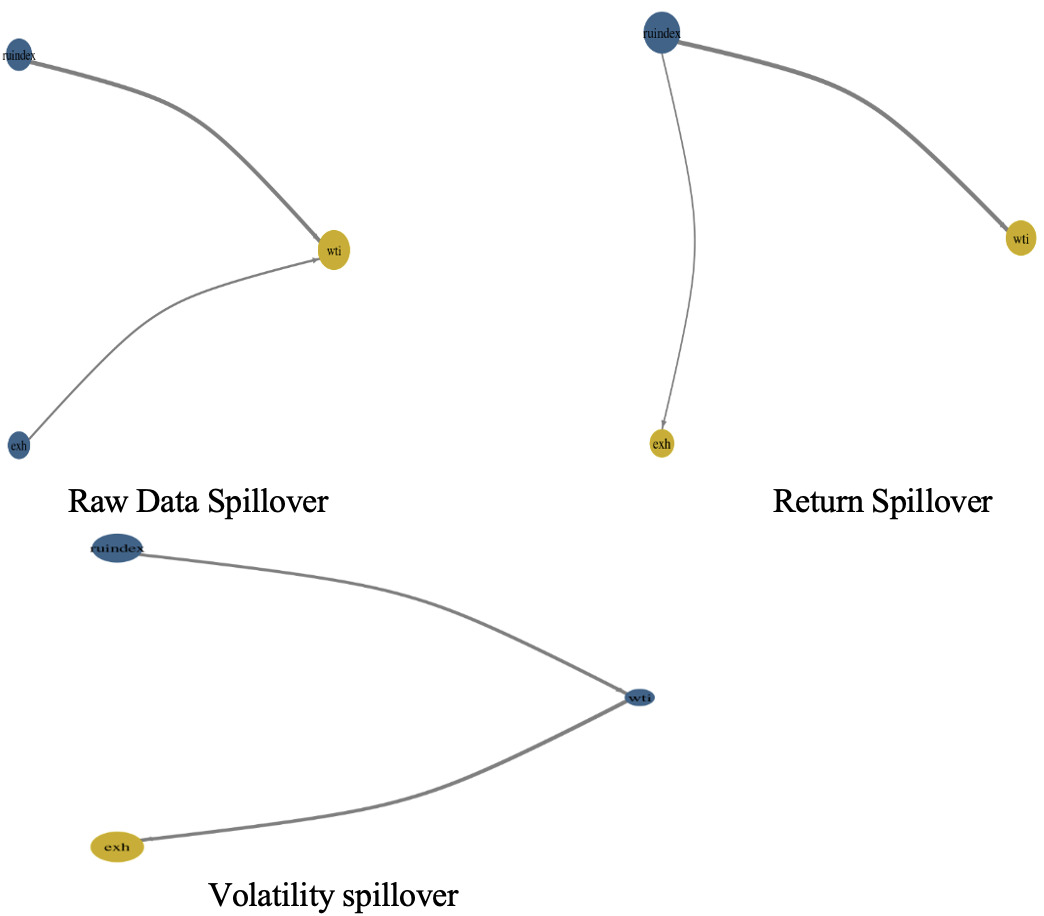
Table 2 presents the dynamic connectedness measures derived from the TVP-VAR model. The findings indicate that spillovers within the RUindex accounted for the largest portion of forecast error variance, as evidenced by the higher values of the diagonal elements relative to the off-diagonal elements. Additionally, the total connectedness index (TCI) reflects the average impact that all variables exert on the forecast error variance of a single variable over time. The TCI across all variables was recorded at 9.26%, as detailed in Table 2. Moreover, the analysis revealed that the RUindex had the most significant impact on the forecast error variance of other variables, with a transmission index of 12.28%, followed by the exchange rate at 11.95%, and WTI at 3.54% (Table 2). The results also highlight the variables that experienced the highest levels of spillovers from other markets, with WTI receiving 15.05%, the exchange rate 7.55%, and the RUindex 5.16%. The final row of Table 2 illustrates the net spillovers for each variable, indicating that WTI was a net recipient of spillovers from other variables, while the remaining variables were predominantly net transmitters.

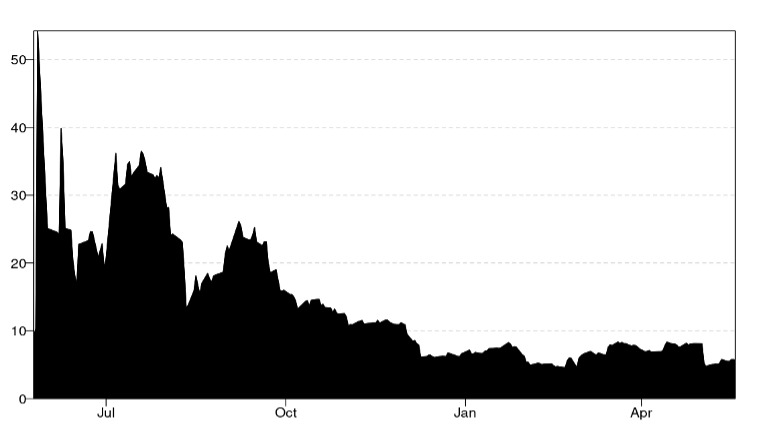
The dynamic total connectedness index (TCI), illustrated in Figure 1, revealed significant fluctuations throughout the entire sample period. Notably, the TCI remained relatively high and recorded its lowest values in mid-January 2023 and April 2023. In contrast, during the first quarter of July 2022, coinciding with the outbreak of the Russia-Ukraine war, the index recorded its highest values. In summary, the network nodes, shown in Figure 2, confirm the results in Table 2. WTI received substantial shocks from the RUindex and exchange rate. Our findings align with those of Ohikhuare (2023) and Shaik et al. (2023).

Figure 1.Dynamic total connectedness.

Notes: The black shaded area illustrates the TCI with external spillovers whereas the light-white line illustrates the internal TCI. Results are based on a TVP-VAR (0.99,0.99) model with lag length of order 1 (BIC) and a 10-step-ahead forecast.

Figure 2.Network diagram

Notes: The blue circles in the graph illustrate the variable(s) whose volatility spills over to others, whereas the yellow circles illustrate the variables that receive volatility spills. The arrows in the graph indicate the direction of the volatility spills and the thickness of the lines along with the arrows indicates the magnitude of the volatility spills.

IV. Conclusion

The movement of oil prices provides valuable insights into the level of risk for market participants. For rational, risk-averse agents, geopolitical risks may prompt a diversification of portfolios in favor of less risky assets. Thus, examining the dynamic connectedness between the Russia-Ukraine war and oil prices holds significant policy implications, which is the primary focus of this study.

The novelty of this research lies in two areas: (i) we analyzed the dynamic connectedness in the nexus between the Russia-Ukraine conflict and oil prices using the innovative Antonakakis and Gabauer (2017) TVP-VAR model. The estimation results indicated a significant degree of connectedness between the Russia-Ukraine war and oil prices. This finding suggests that oil prices are highly susceptible to geopolitical risks such as the Russia-Ukraine conflict.

We are confident that these results, along with the information provided, will enhance the hedging strategies of economic agents and inform the policy decisions of monetary authorities. It is crucial to adopt a more flexible approach when developing investment management strategies and to implement diversified investment portfolios to mitigate associated risks.