Energy Efficiency, Emission Energy, and the Environment

Anelí Bongers

doi:10.46557/001c.13186

1. Introduction

The aim of this paper is to study the implications of technological change in explaining the relationship between the economy, energy consumption, and emissions. Energy consumption is the main source of greenhouse gas emissions into the atmosphere. Two principal technological changes affect the relationship between energy consumption and emissions: energy efficiency technologies and emission efficiency technologies. Although these two environmental quality policies are interchangeable and have similar consequences for the control of emissions, they refer to different technologies, as the former affects the consumption of energy per unit of output whereas the latter affects the emissions per unit of energy used. Our hypothesis is that it could be the case that both technologies have different effects on energy consumption, output, and emissions, and hence, this should be taken into account in the design and implementation of environmental policies promoting energy and emissions efficiency.

This paper contributes to the literature by developing an Environmental-Dynamic Stochastic General Equilibrium (E-DSGE) model in which two types of technologies related to energy consumption and emissions are considered: a technology that improves energy use efficiency (i.e., more energy-efficient engines) and a technology that reduces the quantity of emissions as a function of the quantity of energy (i.e., catalytic converters, particulate filters, etc.). The implications of energy efficiency have been studied using a variety of approaches; see for instance Frondel et al. (2012) and Gillingham et al. (2016). However, little attention has been paid by the literature to study the effects of emissions efficiency. This paper attempts to fill this gap by studying both technologies in an integrated E-DSGE framework. The model considers a three-input production function, namely, physical capital, labor and energy. The stock of pollutants is an externality affecting the final output negatively (see Heutel, 2012; Nordhaus, 2008). The model is calibrated to the US economy.

First, we study the implications of an energy use efficiency technological shock. Energy efficiency technology does not only provoke the well-known “rebound effect” (Frondel et al., 2012; Gillingham et al., 2016), which implies that the positive initial effect of a technological

improvement in energy efficiency leads to the saving of less energy than initially expected. We also find that technological change increases energy consumption, the so-called “backfire effect” (Gillingham et al., 2016; Sorrell, 2009), in production activity in a context in which pollution damages the aggregate productivity. Energy intensity reduces as energy efficiency increases, but the level of emissions also increases and hence energy efficiency policies may be harmful to the environment, as they incentivize energy consumption. Second, we find that a technological improvement in emissions also increases energy consumption but that the effects on emissions are negative, as the reduction in emissions per unit of energy is larger than the increase in emissions due to the higher energy consumption.

In sum, we find that energy consumption increases following both energy efficiency and emission efficiency policies. This is explained by the change in the relative price of energy with respect to the productivity cost of pollution. However, the effects on emissions are different depending on the policy, increasing pollutant emissions with the former and declining emissions with the latter. As a policy recommendation, authorities should incentivize the use not of more efficient energy technologies but of technologies that reduce the level of emissions per unit of energy.

The rest of the paper is structured as follows. Section 2 presents an environmental DSGE model including energy as an additional input factor to capital and labor. Section 3 calibrates the model. Section 4 studies the dynamic properties of the model with regard to two alternative technological shocks. Finally, Section 5 presents some conclusions.

2. An environmental DSGE model with energy

This paper extends the standard Real Business Cycle (RBC) model by Kydland & Prescott (1982) where technological change is the main factor driving economic dynamics and develops an E-DSGE model with a three-input (physical capital, labor and energy) production function.. We assume that, for production, a certain amount of energy must be used and that the use of energy produces pollution. We follow Nordhaus (2008), Heutel (2012) and Golosov et al. (2014) and assume that climate change damages the environment and hence production by reducing productivity.

2.1. Households

The economy is populated by an infinitely lived representative agent who maximizes the expected value of her lifetime utility. Households obtain utility from consumption and leisure. The household utility function is defined as:

$U\left( C_{t},L_{t} \right) = \frac{C_{t}^{1 - \gamma}}{1 - \gamma} - \omega\frac{L_{t}^{1 + \frac{1}{v}}}{1 + \frac{1}{v}}\hspace{15mm}(1)$

where $C_{t}$ is consumption, $L_{t}$ is working hours, $\gamma$ is a risk aversion parameter, $v$ is the Frisch elasticity of the labor supply and $\omega > 0$ represents the willingness to work. We consider a centralized economy. The budget constraint is defined as:

$C_{t} + I_{t} + P_{E,t}E_{t} = Y_{t}\hspace{27mm}(2)$

where $I_{t}$ is investment in physical capital, $Y_{t}$ is the final output (total income), $E_{t}$ is energy, and $P_{E,t}$ is the price of energy, which is assumed to be exogenous.

Investment accumulates into physical capital. The physical capital stock accumulation equation is defined as:

$K_{t} + 1 = \left( 1 - \delta_{K} \right)K_{t} + I_{t}\hspace{20mm}(3)$

where $K_{t}$ is the capital stock and $\delta_{K}\ (0 < \delta_{K} < 1)$ is the depreciation rate of physical capital.

2.2. Pollution

In the literature, a variety of papers assume that emissions are a function of output (see Angelopoulos et al., 2010, 2013; Annicchiarico & Di Dio, 2015; Fischer & Springborn, 2011; Heutel, 2012). However, a more realistic assumption is that emissions are generated by the use of energy in the final production. In particular, we assume that emissions, $X_{t}$ , are proportional to the quantity of energy used:

$X_{t} = nA_{t}^{X}E_{t}\ \hspace{35mm}(4)$

where $n > 0$ represents the carbon content of energy, and $A_{t}^{X}$ is an emission-saving technology. Emissions accumulate into stock pollution, $Z_{t}$ , through the following process:

$Z_{t + 1} = \left( 1 - \ \delta_{Z} \right)Z_{t} + X_{t}\hspace{18mm}(5)$

where $\delta_{Z},(0 < \delta_{Z} < 1)$ is the stock of pollutants’ decay rate.

2.3. Production technology

The model considers a three-factor aggregate production function: physical capital, labor and energy. We assume the following aggregate production function, which exhibits constant returns to scale on all factors, represented by a Cobb–Douglas production function:

$Y_{t} = exp( - \varnothing Z_{t})K_{t}^{\alpha_{1}}{(A_{t}^{E}E_{t})}^{\alpha_{2}}L_{t}^{1 - \alpha_{1} - \alpha_{2}}\hspace{5mm}(6)$

where the term $exp ( - \varnothing Z_{t})$ represents the cost of the damage of pollutants measured as forgone output and $\varnothing > 0$ is a parameter governing the elasticity of aggregate productivity with respect to the stock of pollutants. The final output is influenced by an energy efficiency technology component $A_{t}^{E}$ , and by an externality due to emissions.

Finally, to close the model, we assume that technologies follow a first-order autoregressive process:

$\log A_{t}^{X} = \rho_{x}\log\left( A_{t - 1}^{X} \right) + \varepsilon_{t}^{X}\hspace{18mm}(7)$

$\log A_{t}^{X} = \rho_{E}\log\left( A_{t - 1}^{X} \right) + \varepsilon_{t}^{E}\hspace{18mm}(8)$

Where ( $\rho_{x} < 1,\ \rho_{E} < 1)$ are the persistence parameters and $(\varepsilon_{t}^{X},\varepsilon_{t}^{E}$ ) are i.i.d. innovations in the stochastic processes.

2.4. Centralized equilibrium

The central planner solution is derived by choosing the path for consumption, labor, capital, energy and the stock of pollution to maximize the sum of the discounted utility subject to resource, technology and emission constraints. From the first-order conditions for the centralized problem, we obtain the following equilibrium conditions:

$\text{ωL}_{t}^{\frac{1}{v}} = C_{t}^{- \gamma}(1 - \alpha_{1} - \alpha_{2})\frac{Y_{t}}{L_{t}}\hspace{16mm}(9)$

$\frac{C_{t}^{- \gamma}}{C_{t + 1}^{- \gamma}} = \beta\left\lbrack \left( 1 - \delta_{k} \right) + \alpha_{1}\frac{Y_{t + 1}}{L_{t + 1}}\ \right\rbrack\hspace{10mm}(10)$

$Y_{t + 1} = \frac{C_{t}^{- \gamma}(P_{\text{E.t}} - \alpha_{2}A_{t}^{E}\frac{Y_{t}}{L_{t}})}{\beta C_{t + 1}^{- \gamma}\varnothing nA_{t}^{X}} - \frac{\left( P_{E.t + 1} - \alpha_{2}A_{t + 1}^{E}\frac{Y_{t + 1}}{L_{t + 1}} \right)}{\varnothing nA_{t + 1}^{X}}(1 - \delta_{Z})\hspace{3mm}(11)$

Where $\beta$ is the discount factor. Expression (9) is the optimal labor supply, expression (10) is the optimal consumption path, and expression (11) is the equilibrium condition for the use of energy, representing the optimal stock of pollution that maximizes social welfare.

3. Data and Calibrations

This section presents the calibration of the model’s parameters. Since the model is composed of macroeconomic parameters and parameters related to energy and emissions, we use different sources for its calibration. The macroeconomic parameters are calibrated from the real business cycle literature, while the energy and emission parameters are taken from studies related to the environment and climate change, mostly from Nordhaus (2008), Heutel (2012) and Golosov et al. (2014). The discount factor (for annual data) is fixed to 0.975, whereas the relative risk aversion parameter is equal to 1.2, consistent with the literature. The parameter value (0.33) for the labor supply are selected just to replicate the observed fraction of time devoted to working activities. For the Frisch elasticity of the labor supply, $v$ , we use the value of 0.72, as proposed by Heathcote et al. (2010). The production function technological parameters are taken from the EIA (U.S. Energy Information Administration). We assume that the fraction of labor compensation in the total income is 0.65. As the production function assumes the existence of constant returns to scale, the sum of the technological parameters for the other two inputs, capital and energy, must be 0.35. The technological parameter governing the elasticity of output with respect to energy is obtained from the proportion of energy consumption over the GDP and is estimated to be 0.0982. Therefore, the elasticity of output with respect to physical capital is 0.2518. Finally, the environmental parameters are taken from Nordhaus (2008) and calibrated simultaneously to produce a loss of productivity of 1% in the steady state. The pollution decay rate is fixed at 0.012, as is standard in the literature. Heutel (2012) estimates an elasticity of emissions with respect to output of 0.696, and a productivity loss from pollution of 0.26%. We normalize the emission parameter to 1, resulting in a pollution damage parameter of 0.0087. A summary of the parameters’ calibration is presented in Table 1.

Table 1.Calibration of the parameters

	Parameter	Definition	Value
Preferences	β	Discount factor	0.97
	γ	Risk aversion	1.2
	ω	Labor weight	15.6
	β	Frisch elasticity parameter	0.72
Technology	α ₁	Output–capital elasticity	0.2518
	α ₂	Output–energy elasticity	0.0982
	δ _k	Physical capital depreciation rate	0.06
Environment	n	Emission parameter	1
	δ _z	Pollutant stock decay rate	0.012
	⌀	Pollution damage parameter	0.00875

This table reports the parameters, their description and their values as used in the calibration. The parameter values are obtained from Nordhaus (2008), Heutel (2012), Golosov et al. (2014), Heathcote et al. (2010) and EIA.

4. Results and Discussion

The calibrated model is used to investigate how the economy and the environment respond to energy efficiency and emission efficiency technological shocks. First, we study the response of the economy to a shock that increases energy efficiency. Energy use efficiency refers to technological changes that reduce the amount of energy needed to produce a given quantity of goods and services. The implications of energy-saving technological change on the economy have been studied, for instance, by Newell et al. (1999). They find that energy price changes are the main driving force for energy efficiency technological change.

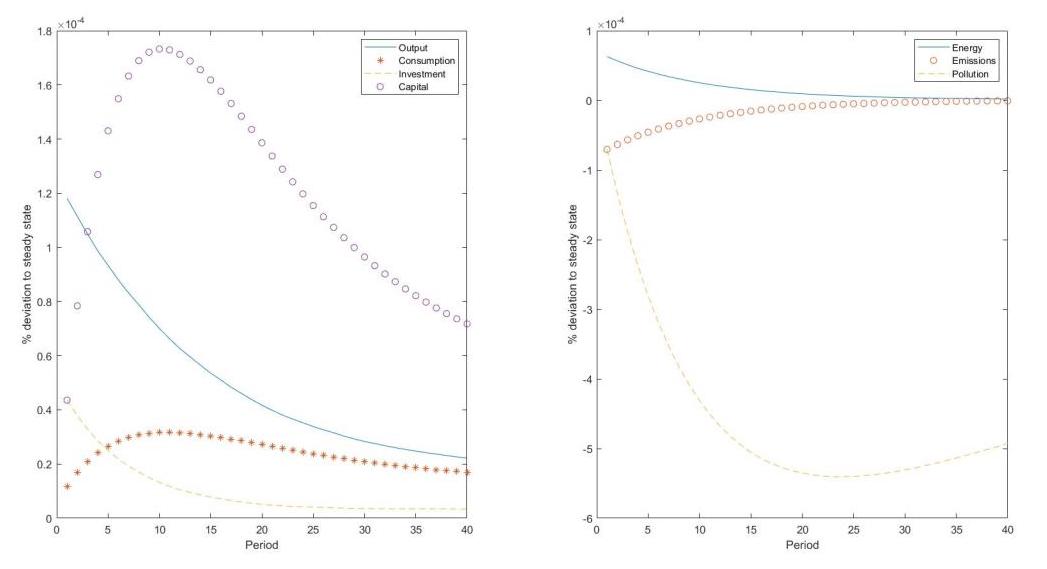
Figure 1 plots the impulse response functions of the main variables of the model to an energy efficiency technological shock. As expected, the response of the output to this shock is positive, as the shock increases the productivity of energy increases. As a consequence, the response of consumption and investment is also positive, indicating that this efficiency technology shock increases physical capital accumulation. The rise in energy efficiency leads to an increase in the demand for energy. However, the increase in the user cost of energy provoked by the pollution externality cost is smaller than the reduction in the user cost of this energy source due to the improvement in energy efficiency, resulting in a final increase in the quantity of energy used in production and in emissions.

Figure 1.Impulse response functions to an energy efficiency technological shock

This figure is based on a model simulation covering 40 periods. Impulse-responses are calculated as percentage deviation of each variable with respect to the steady state.

This result is consistent with the so-called “rebound effect” or “take-back effect” described in the literature on energy efficiency, whereby gains in energy efficiency save less energy than expected (Dimitropoulos et al., 2016; Herring, 2006; Small & Van Dender, 2007). There is also support for the “backfire” hypothesis (Gillingham et al., 2016; Sorrell, 2009), according to which energy efficiency improvements lead to an increase in energy use, an effect derived from the optimal response of economic agents to a technological improvement in energy efficiency, leading to a rise in energy consumption. We also observe that a technological shock provokes a rise in the quantity of energy used in the production activity. The resulting “backfire effect” generates a negative effect on the environment, as the technological improvement in energy efficiency implies a rise in the emission of pollutants.

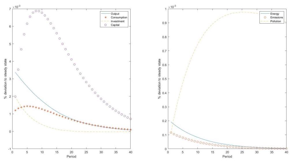
Next, we study the implications of a technological change that reduces the emissions per unit of energy. In this case, the technological change affects not energy efficiency but emission efficiency, having a direct positive impact on productivity. As shown in Figure 2, the output increases in response to this technological shock. This change in the total output results in a rise in consumption and investment, fostering capital accumulation. The explanation is similar to the energy efficiency case, as the shock reduces the relative price of energy by reducing the negative impact of pollution on productivity, but the transmission channel differs. Importantly, the amount of energy used in production increases but with a lower level of emissions, reducing the stock of pollution.

Figure 2.Impulse response functions to an emission efficiency technological shock

This figure is based on a model simulation covering 40 periods. Impulse-responses are calculated as percentage deviation of each variable with respect to the steady state.

Comparing the two environmental policies, we find that they have very different impacts on the environment. The explanation is as follows. An energy efficiency (energy-augmenting) technological shock is equivalent to a reduction in the user cost of energy, increasing the quantity of energy used in production and hence the level of emissions. By contrast, an emission efficiency shock does not change the user cost of energy but directly reduces the productivity losses caused by emissions. In both cases, the optimal response of the economy is to increase energy consumption, but, whereas the higher energy use implies an increase in emissions in the first case, the increase in energy consumption is offset by the lower level of emissions per energy unit in the second case. Finally, we have carried out a sensitivity analysis and found that results are robust to the range of plausible values of the main parameters of the model.

5. Conclusions

This paper studies the effects of energy efficiency and emissions efficiency and their consequences for the environment. We find that they have distinct effects on the environment. Energy efficiency technological change leads to the “backfire effect,” increasing energy consumption, and resulting in a higher level of pollution. By contrast, an emission efficiency technological shock reduces the productivity cost of pollution leading to higher energy consumption but a lower level of emissions per energy unit. This reduces the stock of pollution. The results obtained in this paper indicate that efforts should be put into developing environmental policies fostering emission efficiency and not energy efficiency.