Which Components of Oil Prices Predict Inflation Rate? New Evidence From a Small Island Country, Fiji

I. Introduction

Forecasting inflation is the subject of intense research in macroeconomics. The search for successful predictors of inflation is an exercise that has implications for not only inflation targeting but macroeconomic stability. There is a growing literature on forecasting/predicting inflation rates (see Bec & De Gaye, 2016; Gao et al., 2014; Neely, 2015). The motivation for this literature to investigate the oil price inflation nexus is rooted in household expectations of inflation which they revise every time there is an increase in oil prices or its constituents.

With the importance of oil to macroeconomic stability and economic growth, a sub-set of the literature on forecasting inflation treats oil prices as a predictor. Several studies, as a result, show that oil prices predict inflation. See studies such as Salisu et al. (2017) and Salisu and Isah (2018). A feature of these studies is that they are based on either emerging markets or large developed or developing countries. In this literature, therefore, smaller island economies, where inflationary pressures are equally if not more relevant, are almost always ignored. One such country is Fiji Islands, an island economy which is a leader country in the South Pacific, where growing oil prices have exerted fiscal pressures, leading to debt sustainability concerns.

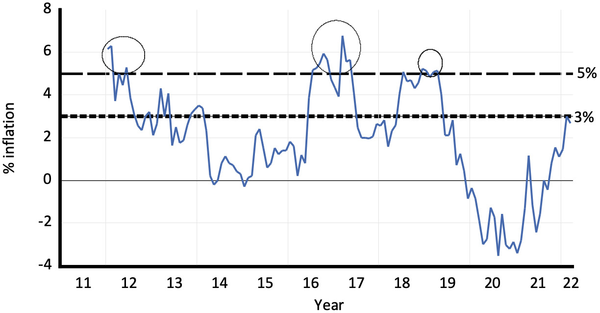
Our contribution to understanding Fiji’s macroeconomic stability is from the point of view of inflation. We attempt to understand what precise role oil price and its constituents, such as diesel, premix, kerosene, and motor spirit play in shaping Fiji’s inflation rate. This is important to investigate because inflation in Fiji has exceeded the 3-5% inflation target rate (see Figure 1). As noted in Narayan et al. (2023) the Reserve Bank of Fiji aims to maintain inflation around the 3-5 percent band.

Figure 1.Annualized inflation for Fiji, 2011 to 2022

Figure 1 represents the annualized inflation rate for Fiji computed from the consumer price index over the period 2011 to 2022.

Using a time-series predictability model developed by Westerlund and Narayan (2012, 2015) that deals with data persistency and model endogeneity and heteroskedasticity we document that: (a) oil prices and kerosene do not predict Fiji’s inflation rate; diesel prices predict a net 0.43% increase in Fiji’s inflation from every one dollar increase in diesel prices and this effect translates over the first 3 months of the price increase; (c) a one dollar increase in the price of premix predicts an increase in Fiji’s inflation rate by 2.27%; and (d) a one dollar increase in the price of motor spirits predicts an increase in inflation of 2.71%.

II. Econometric Framework

The time-series predictive regression model has the following form

$${INF}_{t} = \propto + \beta{Price}_{t - 1} + \rho\mathrm{\Delta}{Price}_{t} + e_{INF,t} \tag{1}$$

In this relationship, INF is the percentage change in the consumer price index obtained from the Reserve Bank of Fiji and Price are proxies for the oil market namely the crude oil price, diesoline, kerosene, premix and motor spirit. Westerlund and Narayan (2012, 2015) show that the general form of Equation (1) is sufficient to address: (a) any predictor persistence, which we estimate using a first order autoregressive model obtained using ordinary least squares, (b) endogeneity which we obtain the regressing the residuals from a regression of INF on one period lagged Price variable on the residuals from a 6^th order autoregressive model of the Price variable and the null hypothesis of no endogeneity is associated with the resulting slope coefficient from the residual-regressed model., and (c) heteroskedasticity, which we address by estimating the predictive regression using a GARCH (1,1) model where errors are assumed to follow a t-student distribution.

The regressions are based on monthly data that covers the sample January 2011 to March 2022.

III. Results

We start with Table 1 which reports some basic information on the data series, the evidence of which paves the way for a formal test of how well inflation can be predicted using oil price, diesel, premix, kerosene and motor spirit.

The first takeaway from Table 1 is about the integration property and persistency of the data, which are captured using the Narayan and Popp (NP, 2010) structural break unit root test and an AR(1) model of the variable, respectively. The NP test rejects the null hypothesis of a unit root with two structural breaks, suggesting that the variables are stationary. The AR(1) model is useful to judge persistency particularly for stationary variables because stationarity is not a sufficient condition for low persistency and if persistency in predictor variables is high, predictive models need to account for it. For all the predictor variables, we find the persistency to be high, in the 0.92 to 0.98 range, with a t-statistic in the 26.73 to 48.22 range.

The endogeneity test reveals that we can only reject the null hypothesis that the slope coefficient in a regression of the residuals from a regression of INF on one period lagged Price variable on the residuals from a 6^th order autoregressive model of the Price variable can only be rejected in the case of oil price (t-stat. = 2.75) but not for the other constituents of oil price.

The heteroskedasticity test is based on a 6^th order autoregressive model of the Price variable and INF. The null hypothesis of no heteroskedasticity is based on the residuals of this model. Except for the INF model, the null hypothesis of no heteroskedasticity is strongly rejected for all Price variable-based models. This result implies that all Price variables are heteroskedastic.

In our first regression, we estimate if oil prices predict Fiji’s inflation. The basic model results are as follows:

$$\begin{aligned} {INF}_{t} &= \binom{0.03}{(0.14)} + \binom{0.001*{OP}_{t - 1}}{(0.70)}\\ & \quad + \binom{0.01*\mathrm{\Delta}{OP}_{t - 1}}{{(2.32)}^{**}} + e_{OP,t} \end{aligned}$$

In this predictive regression, we find that null hypothesis of no predictability cannot be rejected as the OP variable carries a t-statistic of only 0.70. Thus, OP cannot predict Fiji’s inflation. An additional possibility for predictability could be that while one-month lagged OP does not predict inflation, this evidence may change at higher lags. To explore this possibility, we estimate a 6-lag model and obtain the following result:

$$\begin{aligned} {INF}_{t} &= \binom{0.02}{(0.09)} + \binom{- 0.001*{OP}_{t - 1}}{( - 0.26)} + \binom{- 0.00*{OP}_{t - 2}}{( - 0.07)}\\ & \quad + \binom{0.00*{OP}_{t - 3}}{(0.44)} + \binom{- 0.00*{OP}_{t - 4}}{( - 0.04)}\\ & \quad + \binom{0.002*{OP}_{t - 5}}{(0.18)} + \binom{- 0.002*{OP}_{t - 6}}{( - 0.44)}\\ & \quad + \binom{0.01*\mathrm{\Delta}{OP}_{t - 1}}{{(2.28)}^{**}} + e_{OP,t} \end{aligned}$$

From this predictive regression model, we see that the null hypothesis of no predictability cannot be rejected at any of the six lags, suggesting that oil prices do not have any predictive power to influence Fiji’s inflation. This stands in contrast to the literature from other countries where oil price is found to predict inflation. That oil price does not predict inflation may simply mean that there maybe other constituents of oil, such as diesel, premix, kerosene and motor spirit, that may be more relevant to inflation in Fiji. To explore this possibility, the next predict regression takes diesel prices as a predictor variable and obtains the following result:

$$\begin{aligned} {INF}_{t} &= \binom{0.15}{(0.38)} + \binom{0.02*{DIS}_{t - 1}}{(0.09)}\\ & \quad + \binom{- 0.34*\mathrm{\Delta}{DIS}_{t - 1}}{{( - 0.37)}^{**}} + e_{DIS,t} \end{aligned}$$

The null hypothesis that diesel does not predict Fiji’s inflation cannot be rejected with a t-statistic of 0.09. We then test if predictability has a longer horizon effect.

$$\begin{aligned} {INF}_{t} &= \binom{0.24}{(0.59)} + \binom{- 0.47*{DIS}_{t - 1}}{( - 0.53)} + \binom{2.45*{DIS}_{t - 2}}{(1.87)}\\ & \quad + \binom{- 2.02*{DIS}_{t - 3}}{( - 2.23)} + \binom{- 0.18*\mathrm{\Delta}{DIS}_{t}}{{( - 0.18)}^{**}} + e_{DIS,t} \end{aligned}$$

From this regression, we find that the null hypothesis that diesel does not predict inflation is rejected at the 6% level (with a t-stat = 1.87) at the second month, but part of this positive effect on inflation is reversed by the third month (-2.02, t-stat. = -2.23). This means that with every dollar (FJD) increase in diesel, inflation at t-2 increases by 2.45% and declines by 2.02% in month t-3. This represents a net inflationary effect of 0.43% due to every dollar increase in diesel price and this effect is felt in the first 3 months of a price increase.

Next, we consider the predictive strength of premix. Using its price as predictor, we obtain the following result:

$$\begin{aligned} {INF}_{t} &= \binom{0.14}{(0.37)} + \binom{0.02*{PM}_{t - 1}}{(0.11)}\\ & \quad + \binom{- 0.18*\mathrm{\Delta}{PM}_{t - 1}}{{( - 0.23)}^{**}} + e_{PM,t} \end{aligned}$$

$$\begin{aligned} {INF}_{t} &= \binom{0.05}{(0.11)} + \binom{- 1.42*{PM}_{t - 1}}{( - 1.29)} + \binom{2.27*{PM}_{t - 2}}{(1.71)}\\ & \quad + \binom{0.08*\mathrm{\Delta}{PM}_{t}}{(0.10)} + e_{PM,t} \end{aligned}$$

From these regressions, we see that the null hypothesis of no predictability is only rejected at the second month, suggesting that every one dollar increase in the price of premix predicts at increase in inflation by 2.27%.

The next objective is to estimate the predictive power of kerosene and the following results are found:

$$\begin{aligned} {INF}_{t} &= \binom{- 0.12}{( - 0.39)} + \binom{0.20*{KER}_{t - 1}}{(0.94)}\\ & \quad + \binom{0.29*\mathrm{\Delta}{KEAR}_{t - 1}}{(0.45)} + e_{KER,t} \end{aligned}$$

$$\begin{aligned} {INF}_{t} &= \binom{- 0.01}{( - 0.03)} + \binom{- 0.25*{KER}_{t - 1}}{( - 0.35)} + \binom{0.75*{KER}_{t - 2}}{(0.80)}\\ & \quad + \binom{0.75*{KER}_{t - 3}}{(0.73)} + \binom{- 1.09*{KER}_{t - 4}}{( - 0.94)}\\ & \quad + \binom{0.73*{KER}_{t - 5}}{(0.68)} + \binom{- 0.78*{KER}_{t - 6}}{( - 1.26)}\\ & \quad + \binom{0.38*\mathrm{\Delta}{KER}_{t - 1}}{{(0.61)}^{**}} + e_{KER,t} \end{aligned}$$

We see that neither in the basic model nor in the augmented 6-month lag model there is any evidence that kerosene price predicts Fiji’s inflation.

The final model tests the predict power of motor spirit prices in predicting Fiji’s inflation rate and the following results are obtained:

$$\begin{aligned} {INF}_{t} &= \binom{0.13}{(0.28)} + \binom{0.02*{MS}_{t - 1}}{(0.10)}\\ & \quad + \binom{- 0.41*\mathrm{\Delta}{MS}_{t - 1}}{( - 0.49)} + e_{MS,t} \end{aligned}$$

$$\begin{aligned} {INF}_{t} &= \binom{0.16}{(0.29)} + \binom{- 1.27*{MS}_{t - 1}}{( - 1.12)} + \binom{2.71*{MS}_{t - 2}}{(1.98)}\\ & \quad + \binom{- 1.86*{MS}_{t - 3}}{( - 1.48)} + \binom{0.41*{MS}_{t - 4}}{(0.25)}\\ & \quad + \binom{0.52*{MS}_{t - 5}}{(0.33)} + \binom{- 0.52*{MS}_{t - 6}}{( - 0.59)}\\ & \quad + \binom{- 0.43*\mathrm{\Delta}{MS}_{t - 1}}{{( - 0.46)}^{**}} + e_{MS,t} \end{aligned}$$

From these results, we find predictability at the second month horizon. That is, at t-2, we find that motor spirit prices positive predict Fiji’s inflation with an effect of 2.71 (t-statistic = 1.98). This implies that for every one dollar increase in motor spirit prices, inflation increases by 2.71% and this result is statistically significant at the 5% level.

IV. Concluding Remarks

This note explores the role of oil prices and its constituents (namely, diesel, premix, kerosene, and moto spirit) in predicting Fiji’s inflation rate. The literature has documented the importance of oil prices to inflation. We should that while oil prices may predict inflation for larger economies, as the literature has shown, this is not true for small island states such as Fiji. For such economies, it is the other constituents of the oil market that matter. In Fiji’s case, we find that oil price does not predict inflation, but diesel, premix and motor spirits predict inflation by between 0.43% to 2.71%.