A Letter on the Distributional Impact of Electricity Subsidies in Argentina: Conceptual Framework and Measurement

I. Introduction

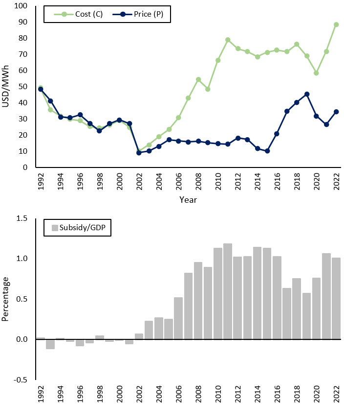
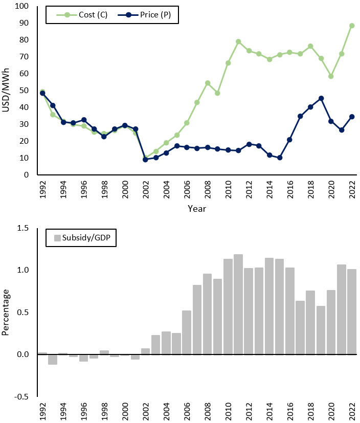
In this letter, we review the distributional impact of electricity subsidies. We use the attractive case of Argentina, which presents a rich background in terms of how electricity prices have been implemented with the objectives of improving income distribution, controlling inflation, and promoting economic growth, among other policy goals (Cont et al., 2021). In recent decades, Argentina has massively subsidized electricity: from 0.1 percent of GDP in 2002, electricity subsidies rose to 1.1 percent in 2015 and in 2022 stood at 1.0 percent (see Figure 1). In fact, Argentina ranks among the top 25 ranking of energy subsidiaries (IEA, 2022). During this period, attempts to decrease high subsidies generated strong reactions that led to reversing course (e.g., see years 2019 to 2022 in Figure 1).

The subsidy policy has generated a lot of academic research that unanimously highlights a singular distributional result: subsidies are progressive as poorer sectors receive higher subsidies relative to their income (Giuliano et al., 2020; Hancevic et al., 2016).^[1] Interestingly, the empirical consensus presents a particularity as it focuses on the subsidies’ incidence without considering government financing. In this letter, we address this issue, focusing on subsidies for residential consumption.

We show that government financing is a central dimension for better understanding the subsidies’ distributional effects. As Musgrave (1964) emphasized many decades ago, “... [a]ny meaningful theory or policy in public finance must ultimately combine the issues posed by the two sides of the budget. This, indeed, is the cardinal principle of the economist’s view of public finance”. It is common to treat public programs and taxes separately, but the importance of analyzing them together is clear. For example, if a program is progressive but its financing is very regressive, income inequality may increase after the program is implemented (Gasparini et al., 2014).

We first develop a simple conceptual framework following the literature on the design of prices for public services (M. Feldstein, 1972; M. S. Feldstein, 1972). The subsidy is defined as the departure of prices from production costs. Second, combining household survey micro-data with sectoral administrative data (i.e., prices and costs of electricity), we measure the subsidy at the household level and perform a distributional analysis (Van de Walle, 1998). To align with previous literature, we initially do not consider government financing, and we confirm the consensus: subsidies are progressive. Then, we simulate that the government finances the subsidy with a general consumption tax, and we find relevant results: the progressivity is strongly attenuated.

The letter is informative for existing literature on energy subsidies in other countries (Dartanto, 2013; Rosas-Flores et al., 2017). It also contributes to previous works analyzing the role of energy prices in redistributing income even in the absence of subsidies (Levinson & Silva, 2022). The letter is also accurate and timely as energy subsidies (i.e., electricity and natural gas) have been a key topic in Argentina’s recent times,^[2] and they were especially prominent in public discussion during the 2023 Presidential election. Furthermore, the president-elect recently implemented a subsidy reduction in 2024.^[3]

II. Conceptual Framework

Electricity is consumed by \(j\) individuals \((j = I,\ldots,J)\). The marginal cost of production (i.e., \(c_{e}'\)) equals the average cost and is the same for all users. The price is different for each user due to different costs of distribution (i.e., \(p_{ej}\)). The electricity subsidy is defined as the departure of \(p_{ej}\) from \(c_{e}'\). It is financed by a general tax on \(i\) goods \((i = 1,\ldots,n)\), uniform to all users. The margin between \(p_{ej}\) and \(c_{e}'\) can be obtained from the following model:

\[\small{\begin{aligned} \max \mathcal{L} & = W\left( v_{j}\left( p_{ej};p_{1},\ldots,p_{n} \right) \right)\\ & \quad + \mu\left\lbrack \sum_{j}{p_{ej}{*q}_{ej}} - \sum_{j}{c_{e}\left( q_{e} \right)} + \sum_{i}{p_{i}*q_{i}} - \sum_{i}{c_{i}\left( q_{i} \right)} \right\rbrack \end{aligned}}\]

As a result,

\[\frac{p_{ej} - c_{e}'}{p_{ej}} = \frac{\sigma_{j} - \mu}{\mu\eta_{ej}}\tag{1}\]

Note that the margin is personalized (at the household level and, consequently, by groups of income) since, although the cost is the same for everyone, the price that each user pays varies according to the price schedule (i.e., uniform prices, tariffs in two or multiple parts, etc.). As is usually the case, the margin depends on the financial restriction (\(\mu\)), the price elasticity of demand \(\left( \eta_{ej} \right)\) and the social marginal value of income for consumer \(j\) \(\left( \sigma_{j} \right)\).

A uniform tax system is assumed. The goods are taxed, and the resulting (price-marginal cost) margin is:

\[\frac{p_{i} - c_{i}'}{p_{i}} = \frac{\mu - d_{i}}{\mu\eta_{i}}\tag{2}\]

where \(d_{i}\) is the distributive characteristic of good \(i\) and it is defined as the sum of users’ social marginal valuations of income weighted by the consumption share of the good (F. Navajas & Porto, 1994). Although the tax system is uniform, the tax collection for different individuals may vary depending on the level of consumption.

III. Measurement and Analysis

Table 1 presents the margins’ measurement for the Buenos Aires Metropolitan Area (i.e., AMBA) just to be on the same page as the previous literature (Giuliano et al., 2020; Hancevic et al., 2016). We use the most recent National Household Income and Expenditure Survey (ENGHo) for 2017 and 2018.

First, we order individuals by per capita household income, and we build deciles (Column 1). Second, following Navajas (2009), we do not use quantities as reported in the survey because they tend to be under-reported. Thus, quantities are retrieved from the expenditure on electricity after deducting taxes and using the tariff charts for final users. Column 2 presents the monthly average consumption at the household level (in per kilowatt hour (Kwh) and per capita terms).

Third, we compute electricity costs, which include generation, transmission, and distribution. Generation and transmission costs are determined in the Wholesale Electricity Market (WEM). Using the peso-per-dollar exchange rate in effect during 2018 (i.e., 28.85 ARS/USD), the unitary cost was 2.2 ARS/Kwh.^[4] Distribution costs are determined by the cost structure of each energy distributor company (i.e., distance to final users, operational efficiency, etc.). Based on data from EDENOR and EDESUR, the two main electricity distributors in AMBA, this cost was 0.9 ARS/Kwh. Thus, the total cost was 3.1 ARS/Kwh (Column 3).

Residential users pay an electricity bill that includes both a fixed and a variable component. Final prices reflect a distributional criterion, as distributors set higher prices for higher consumption levels. Additionally, there is a social tariff for less well-off families.^[5] The eligibility criteria are based on the income level and socioeconomic status of the primary service holder. Then, prices are personalized for each household (Column 4).

Column 5 presents the departure of prices from costs (i.e., equation 1). This deviation primarily occurs in the WEM, as the federal government has been selling electricity below the cost of production since 2002.^[6] As a result of the social tariff subsidy, the margin is higher in the lower deciles. The average subsidy is obtained in Column 6 and the well-established middle to high-income bias is confirmed (Giuliano et al., 2020; Hancevic et al., 2016).

We then consider a government financing scheme, naturally not exhaustive as it is selected to just illustrate a conceptual point. Note that a share of the electricity subsidies is already financed with taxes (i.e., the VAT collected through the electricity bill itself). The remaining—to guarantee balanced budget—is assumed to be financed via general VAT. So, we rely on the standard incidence assumptions: VAT is supported by final consumers as in Fernández Felices et al. (2016). We distribute the tax using the total household expenditure (Column 7). In Column 8, we compute the net subsidy as the difference between the subsidy (Column 6) and the tax (Column 7) for each decile. The contribution of each decile towards financing the subsidy is relevant for understanding its distributional impact.

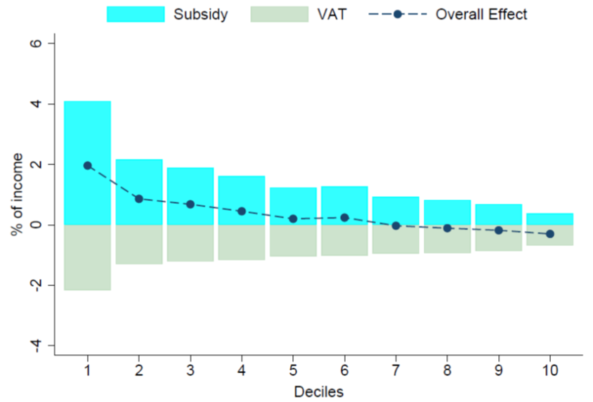
Figure 2 presents the net effect as a share of the income after fiscal policy.^[7] The poorest decile receives, on average, 4.1 percent in terms of electricity subsidies, while it contributes to the financing with 2.2 percent in terms of VAT. In net terms, the poorest decile gains 1.9 percent (i.e., Overall Effect). This is less than half of what it gains solely from subsidies. Note that this benefit’s reduction is true for all deciles and the well-established result on the progressivity of electricity subsidies is strongly attenuated.

A discussion on the welfare effects of subsidies is relevant here when considering a welfare function as defined by Sen & Foster (1973): \(W = y * (1 - G)\); where \(y\) is the average income and \(G\) is the Gini coefficient. Here, W increases with y and decreases with \(G\). When financing is omitted, \(y\) increases and \(G\) improves. However, if financing is included, \(y\) remains constant, and the overall welfare effect depends on \(G\). Thus, understanding how inequality changes is crucial for evaluating the distributional impact of subsidies.

The previous finding can be considered against other financing alternatives. For example, Argentina has had high inflation for more than a decade. Money printing could be considered as another source of financing. Assuming that inflation is regressive, conclusions can be drawn based on this letter’s findings. In the same spirit, a comprehensive distributional analysis should look at subsidies against spending. Higher subsidies can substitute public spending with strong redistributive power such as spending on education (Ebeke & Ngouana, 2015).^[8]

IV. Conclusions

In this letter, we show how omitting subsidies’ financing can lead to a biased belief about their redistributive effect. We support this point with a conceptual framework and microsimulations that combine micro-data at the household level. The application is for the notable case of Argentina, which has massively subsidized electricity in recent decades. The scope of these findings could be useful for other countries dealing with energy subsidies.

Several globally relevant policy recommendations can be drawn from this letter. First, prices set below the marginal cost of provision due to subsidies may not be an effective instrument for income redistribution, as they often result in leakages to higher-income groups. Second, even with leakages, subsidies can be progressive as the subsidy-to-income ratio decreases throughout the income distribution. However, the distributional impact of subsidies should be evaluated by considering both sides of the budget. Finally, analyzing public policies through solid and well-established conceptual frameworks is recommended. This will provide accurate guidance in the analysis and public debate, resulting in well-founded conclusions for sound policy recommendations.

Figure 1.Evolution of prices, costs and subsidies to electricity in Argentina. In dollars and percentage of GDP. Period 1992-2022

Source: Own elaboration based on the Wholesale Electricity Market (WEM) Administration Company (CAMMESA). Annual reports. Note: The price represents the stabilized price of energy (i.e., the price that demand directly pays). The average cost includes generation and transmission (given by the “monomic cost” in the WEM).

Figure 2.Net distributional incidence of electricity subsidies when considering public financing through general VAT. By deciles of per capita income. In percentage of post-fiscal income

Source: Own elaboration based on ENGHo 2017-18 and specific information of the energy sector. Note: All values are weighted using the population expansion factor.

Acknowledgements

We would like to thank Afees Salisu and two anonymous referees. All authors belong to Center of Public Finance Studies (CEFIP), IIE-FCE, National University of La Plata (UNLP). Porto also belongs to National Academy of Economic Science of Argentina (ANCE). Bertín also belong to Center for Distributive, Labor, and Social Studies (CEDLAS), IIE-FCE-UNLP. Pizzi also belongs to UC Davis (California). Jorge Puig also belongs to CEDLAS and Partnership for Economic Policy (PEP). The usual disclaimer applies. Email for contact: jorge.puig@econo.unlp.edu.ar (J. Puig).