Shannon-Wiener Index: Carbon Emission and Energy Consumption Structure in India

I. Introduction

It is known to us that climate change will have an impact on the natural ecosystem and socio-economic system. The phenomenon of environmental degradation, particularly through global warming, can be attributed to the ongoing rise in carbon dioxide (CO₂) emissions. Recent studies, such as Qiao et al. (2020), reported that the surface temperature of the universe has increased by 0.4°C to 0.8°C, and it is predicted that in the 21^st century, this surface temperature will increase by 1–5 °C.

India, the third-largest greenhouse gas emitter globally, faces challenges due to its extensive natural resources and environmental variety. The country’s economy, ranking fourth globally, faces disparities and uneven resource distributions. Investments in agriculture, infrastructure, power, manufacturing, and automobiles have increased significantly, leading to a surge in emissions and pollution. In 2019, India produced 2,597.4 million tons of CO₂ emissions, with an annual rise rate peaking at 11.65% in 2009 before declining to 1.6% in 2019.^[1]

Before projecting future estimates, it is imperative to comprehend the linkages between energy consumption, economic growth, and emissions, especially as CO₂ emissions are primarily driven by anthropogenic factors, particularly activities engrained in fossil fuel-based production. A study by Murthy et al. (1997) on India’s greenhouse gas emissions highlights the complex relationship between economic growth, carbon emissions, and energy demand. The paper predicts a significant rise in India’s CO₂ emissions by 2020 due to economic growth and changing consumption patterns. However, this is lower than in many developed countries. Energy-efficient technologies and policies can help reduce emissions. Environmental degradation worsens with economic growth, aligning with the Environmental Kuznets Curve (EKC) concept. Studies have shown that while nuclear power, hydropower, and other alternative resources have negative effects on CO₂ emissions, the size of the population, per capita GDP, power intensity, and energy consumption have beneficial effects (Noorpoor & Nazari Kudahi, 2015). In 2023, a study by Luqman, Rayner, and Gurney shows that urban CO₂ emissions are increasing globally and indicates a negative correlation between trends in population density and per capita CO₂ emissions. According to this study, urbanization will become a more serious issue for carbon emission. Kim et al. (2019) arrives at the conclusion that while there is no short-term relationship between foreign direct investment and CO₂ emissions, there is a co-integration relationship over the long run between CO₂ emissions, GDP, and foreign direct investment, confirming the existence of EKC based on data from 1980 to 2013 for 57 underdeveloped countries. Azam et al. (2016) found a correlation between economic growth and CO₂ emissions in China, Japan, and the USA. According to Li et al. (2021), trade openness will only raise the carbon emissions of the lower middle-income group, whereas increasing renewable energy consumption helped to reduce carbon emissions. Sun & Ren (2021) investigated the interconnections between CO₂ emissions and energy consumption structure and questioned the applicability of the EKC theory in China. Their study introduced the Shannon-Wiener Index as a novel indicator, considering factors like urban growth, commerce, and energy use structure. The research uncovered that China does not follow an EKC.

The diverse findings underscore the need for nuanced approaches to environmental policies, accounting for the specific economic conditions of individual nations. However, a specific gap remains in the literature concerning the context of India. India’s CO₂ emissions increased by 80 Mt in 2021 due to more coal usage in electricity generation. Despite targeting 40% non-fossil power capacity, the country’s population size raises concerns about future emission growth. The unique socio-economic and environmental factors that characterize India’s meteoric economic rise make it essential to conduct an exhaustive study. Balancing ecological preservation and economic growth is essential for policymakers, particularly in developing nations like India, where globalization has strengthened trade openness. Our study explores how India’s carbon emissions interact with economic development, trade structure, urbanization, and the Shannon-Winner Index. Using the Autoregressive Distributed Lag Bounds (ARDL) test, we aim to uncover correlations among these variables. As research on growing economies is limited, our study on India, a major emerging economy, provides crucial insights. Section II details our data and methodology, section III discusses findings, and Section IV concludes the paper.

II. Data and Methodology

A. Data description and model

In this research article, India’s annual time series data from 1990 to 2021 was used for the investigation. Annual time series data on urbanization rate, ratio of export to import, and GDP per capita (constant 2015 US$) are sourced from the economic database of the World Bank and ourworldindata. The EKC hypothesis postulates an inverted U-shaped relationship between GDP per capita and environmental degradation. Urban areas usually have higher energy demands and increased industrial production, which significantly contributes to carbon emissions. Thus, we consider the urbanization rate (UR) as a crucial factor. Trade specialization (TS) provides insights into a country’s foreign trade dynamics. Countries heavily reliant on certain exports may have different carbon emissions trajectories compared to those with diversified trade portfolios, such as fossil fuels. Shannon-Wiener Index (SWI) measures energy consumption structure. It reveals the impact of clean energy development on carbon emissions, considering the varying carbon emission coefficients of different energy sources.

There is a relationship between quality of environment and per capita income:

\[ E_{i t}=\beta_0+\beta_1 Y_{i t}+\beta_0 Y_{i t}^2+\varepsilon_{i t} \tag{1} \]

This model was first developed by Grossman and Krueger (1995).

Here,

E_it = Per capita carbon emissions,

Y_it = GDP per capita,

ε_it = Error term,

‘i’ and ‘t’ represent countries and year, respectively.

Based on Equation (1), urbanization rate, ratio of export to import, and proportion of coal consumption are introduced as independent variables. We have also introduced SWI in our model to account for the diversity of energy sources (crude oil, natural gas, coal, hydropower, nuclear, wind, and solar; in terawatt-hours) in the renowned relationship.

We have calculated SWI based on the following formula:

\[ S W I=-\sum_{i=1}^n P_i \times \ln \left(P_i\right) \tag{2} \]

SWI indicates the variety of the energy consumption system, where n is the number of different energy types in the energy consumption system and P_i is the energy consumption ratio i.

To examine whether EKC hypothesis is valid in India, the following empirical model has been formed:

\[ \begin{align} C O_2&=\alpha_0+\alpha_1 Y_t+\alpha_2 Y_t^2+\alpha_3 U R_t\\ &\quad+\alpha_4 T S_t+\alpha_5 S W I_t+\epsilon_t \end{align}\tag{3} \]

If we find the coefficient of Y_t and Y_t² are positive and negative, respectively, then we could say that the EKC hypothesis is applicable in India.

In Equation (3),

CO₂ = Per capita carbon dioxide emission in logarithm form,

Y_t = GDP per capita in logarithm form,

Y_t² = (GDP per capita in logarithm form)²,

UR_t = Rate of urbanization,

TS_t = Structure of trade,

SWI_t = Shannon- Wiener Index of energy,

ε_t = Remainder,

and α₁, α₂, α₃, α₄, α₅ = Elasticity of CO₂ of different variables in the logarithm form.

B. Econometric models and methodology

The ARDL model is widely used due to its advantages over other cointegration methods. The ARDL model is suitable for small samples, flexible, and can be analyzed with I(0) and/or I(1) data. Unlike conventional methods, ARDL allows different lag lengths for different variables, and fully addresses autocorrelation and endogeneity issues. Pesaran et al. (2001) further elaborate its application.

We developed an unconstrained error correction model (UECM) based on the ARDL model, that encompasses both long-term and short-term associations between variables.

\[\small{ \begin{align} \Delta LogCO2 &= \delta_{0} + \delta_{1}Log{CO2}_{t - 1} + \delta_{2}LogY_{t - 1} + \delta_{3}Log{Y^{2}}_{t - 1} \\ &\quad+ \delta_{4}{URATE}_{t - 1} + \delta_{5}{TS}_{t - 1} + \delta_{6}{SWI}_{t - 1} \\ &\quad+ \sum_{i = 1}^{p_{1}}\delta_{1i}\Delta Log{CO2}_{t - i} + \sum_{i = 0}^{p_{2}}\delta_{2i}\Delta LogY_{t - i} \\ &\quad+ \sum_{i = 0}^{p_{3}}\delta_{3i}\Delta Log{Y^{2}}_{t - i} + \sum_{i = 0}^{p_{4}}\delta_{4i}\Delta{URATE}_{t - i} \\ &\quad+ \sum_{i = 0}^{p_{5}}\delta_{5i}\Delta{TS}_{t - i} + \sum_{i = 0}^{p_{6}}\delta_{6i}\Delta{SWI}_{t - i} + \epsilon_{1t} \end{align} \tag{4} } \]

In the formula, ϵ_1t, is the Gaussian white noise and ∆ is the first-order difference. Here p is the lag order, which is usually calculated by AIC criterion, whereas δ_i (i = 0, 1, 2, 3, 4, 5, 6) is the long-run coefficient between variables, and δ_ji (j = 0, 1, 2, 3, 4, 5, 6) is the short-run coefficient between variables.

III Empirical Analysis

The ADF test reveals that the p-values for TS, UR, and CS are all below 0.05, indicating stability at the 5% significance level and classification as I(0) processes. Regarding CO₂, GDP, GDP², and SWI, while the original sequences lack stability, the p-value after the first-order difference is below 0.05, signifying the absence of a unit root at the 5% significance level and rendering the series significant at I(1).

A. Results and findings

Based on the data presented in (Table 1), we found that URATE (or UR) positively affects CO₂ emissions in India, supporting concerns about escalating urban CO₂ emissions globally (Luqman et al., 2023). As more people move to cities, energy demand rises due to increased industrialization, transportation, and residential energy use. The TS and SWI negatively affect CO₂ emissions, meaning that diversifying trade and promoting a balanced energy portfolio can help reduce emissions. The adjusted R² value is approximately 0.99 which shows that the experimental model fits well. Hence, our model captures the underlying relationships effectively. The coefficient of LOGY is -10.272, while the coefficient LOGYSQR is 1.803. The symbolic direction shows that EKC hypothesis is not valid in India. The F-statistic value of 4.699 is greater than the upper bounds critical value (4.15) at the 1% level. This indicates a long-run relationship among the variables (Table 2). In other words, changes in these factors have lasting effects on India’s carbon emissions. While previous research has shown a positive relation between economic growth and CO₂ emissions (Azam et al., 2016), our findings indicate the opposite relation. From (Table 3), we found that the significant speed of adjustment parameter (ECT(-1)) is -0.586, indicating that India’s carbon emissions can rapidly transition to a long-run equilibrium state. At the 1% significance level, short-run fluctuation of the per capita GDP significantly impacts the growth rate of India’s per capita CO₂ emissions. A unit change in per capita GDP growth results in a 10.272 unit change in the opposite direction for per capita CO₂ emissions, highlighting the influence of GDP growth on carbon emissions. Contrary to predictions of a significant rise in CO₂ emissions by 2020 due to economic growth (Murthy et al., 1997), our findings suggest a nuanced scenario, perhaps diverging from trends observed in India. As urbanization accelerates, carbon emissions increase rapidly. Additionally, the current trade structure affects CO₂ emissions in the opposite direction, with a significant impact observed when the trade structure lags by one period.

Figure 1.CUSUM test & CUSUMSQ test.

Note: Significant at 5% level. Constant volatility at 5% level.

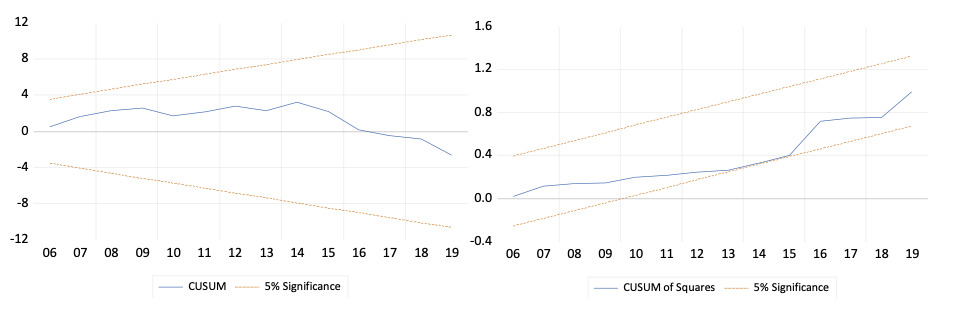
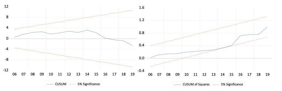
From the findings (Figure 1) of stability tests it is found that both the CUSUM & CUMSUMSQ curves are within the boundary of the dotted line at 5% significance level. This proves that the parameters of the regression equation are stable.

IV. Conclusion and Policy Suggestions

In this article, we have introduced some important factors, such as urban development, trade level and the Shannon-Winner Index. Short-run and long-run relationships are examined by using ARDL model. Overall, the article focuses on the validity of EKC hypothesis in India. From the empirical analysis, the following points can be sought out. The EKC hypothesis is rejected in India. An increase in the SWI will reduce carbon emissions.

These findings suggest that we should endeavor to reduce coal consumption, promote electricity usage, and efficient public transportation systems. We should also reduce reliance on carbon-intensive industries and make an effort to increase investments in clean energy. The government should offer tax incentives and subsidies for electric vehicle purchases, as well as investments in solar, wind, and hydroelectric power.