Oil Prices and Expectations: A Quantile Structural VAR Approach

I. Introduction

Competitive markets allow information flow between market agents. The equilibrium price for such markets is normally upheld such that all available market information are transmitted to the agents (Fama, 1970). The synchrony between price and supply/demand is attained because current and expected information are incorporated by arbitrageurs. However, when there are informational frictions, price and supply/demand may diverge, because the market price vector is dissimilar to the available information vector available to different agents (Hellwig, 1980). Informational frictions in oil markets may cause a dislodge between oil prices and supply and/or demand shocks (Byrne et al., 2019). Geopolitical shocks can also cause oil price to diverge from the fundamentals (Bakas & Triantafyllou, 2020; Caldara & Iacoviello, 2022; Zhang et al., 2022). Consequently, during informational frictions, market participants are oblivious to the different sources of oil shocks, such as supply and demand (Singleton, 2014; Sockin & Xiong, 2015).

Furthermore, acute informational frictions can cause uncertainty among market participants regarding the robustness of the global economy and oil demand in relation to supply (Sockin & Xiong, 2015). Consequently, it may be unrealistic to assume that consumers and producers can observe directly and concomitantly whether oil prices align with fundamentals. Singleton (2014) emphasizes that in the face of informational frictions, differential expectations among investors can cause a wedge in future prices of commodities. Therefore, without a concurrent link between oil prices, fundamentals, and speculation, the role of expectations is critical.

Building on Sockin & Xiong (2015), and Singleton’s (2014) studies, Byrne et al. (2019) incorporated economic agents’ expectations regarding the state of the global economy to identify the underlying influences of oil price changes; business expectations, unlike consumer expectations, play an important role in oil price movements. Additionally, this impact varies over time. For instance, business expectations had a negligible effect on oil prices from the mid-80s throughout the '90s. However, the authors note that from 2002 to 2014, business expectations played an important role in explaining the fluctuation of oil prices. Nevertheless, this impact decreased from 2014 to 2016, which marks the end of their sample period. Regarding consumer expectation, the authors find that the impact is negative, which they regard as a puzzle and mostly time-invariant.

Based on Byrne et al.'s (2019) work, we investigated how unexpected shocks from business and consumer expectations impact oil price distribution. Our results revealed that expectational shocks affect the impulse response of oil price distribution heterogeneously. Specifically, a positive business expectation shock has a positive effect on the mean of oil prices, but its persistence varies based on the quantiles of oil prices. The conditional response of lower oil price quantiles exhibits higher persistence than upper quantiles. In contrast, the existing literature suggests that consumer expectations have a negligible effect on oil prices. However, our findings indicate that this holds true only for the mean reaction of oil prices. When analysing the entire oil price distribution, consumer expectation shocks can have significant and persistent effects on the lower oil price quantiles. Nevertheless, this effect diminishes and loses significance when expectational shocks occur at higher oil prices.

The structure of this paper is outlined as follows: Section 2 introduces the methodological approach and data employed in the study. The findings are discussed in Section III. Finally, Section IV offers concluding remarks.

II. Methodology and Data

A. Global oil market

Since the seminal work of Kilian (2009), the global oil market has been customarily modelled by a recursive structural vector autoregressive (SVAR) framework. This framework identifies different supply and demand shocks that affect the global crude market. Usually, in a recursive order, shocks are labelled as flow supply, flow demand, and oil-specific demand shocks. Flow supply shocks are unexpected events that affect the production or availability of crude oil in the global market. Flow demand shocks are unpredictable innovations to the global demand for crude oil. Oil-specific demand shocks are innovations to the real oil price based on oil market demand.

In this study, we adopted Chavleishvili & Manganelli’s (2023) methodology to estimate quantile recursive vector autoregressive (VAR) models. Quantile regression is well-known in economics and statistics (Koenker, 2017; Koenker et al., 2006; Koenker & Bassett, 1978). Its popularity derives from its ability to estimate robust quantile-specific effects from covariates; therefore, it provides more information than ordinary least squares regressions. Specifically, it facilitates the study of the entire response distribution after a shock in both oil market fundamentals and expectations.

Early applications to time series can be traced back to Engle and Manganelli (2004) and Koenker et al. (2006), who developed the univariate quantile autoregressive model (QAR). Its main advantage is the possibility to model important phenomena in time series, such as, asymmetric response, local persistency, and nonlinearities. The extension to modelling multivariate time series, however, is not trivial and has been the subject of active research. Some recent efforts in this area include reduced form VARs (Montes-Rojas, 2019), Granger causality (Troster, 2018), and structural VARs (SVAR) (Chavleishvili et al., 2021; Chavleishvili & Manganelli, 2017, 2023; Montes-Rojas, 2022; Ruzicka, 2021).

Complying with Byrne et al. (2019), and Chavleishvili & Manganelli’s (2023) studies, the QSVAR model of the global oil market with expectations was specified in Equation 1.

where $\Delta q_t$ represents monthly percentage change in global oil production, $y_t$ is a measurement of real economic activity, $e_t$ represents agent expectation, and $p_t$ is the real oil price. Furthermore, $\varepsilon_t^s, \varepsilon_t^d, \varepsilon_t^e$, and $\varepsilon_t^o$ represent the flow supply, flow demand, expectational, and oil-specific demand structural shocks. $\boldsymbol{x}_{\boldsymbol{t}}=\left(1, \boldsymbol{y}_{\boldsymbol{t}-1}^{\prime}, \boldsymbol{y}_{\boldsymbol{t}-2}^{\prime}, \ldots, \boldsymbol{y}_{\boldsymbol{t}-\boldsymbol{p}}^{\prime}\right)^{\prime}$ with $\boldsymbol{y}_{\boldsymbol{t}}^{\prime}=\left(\Delta q_t, y_t, p_t\right)^{\prime}$. Data definitions are in the next section. Also, error terms satisfy the property that $P\left(\varepsilon_t^j\left(\theta_i\right)<0 \mid \Omega_{i t}\right)=\theta_i$ with $i=1, \cdots, 4$, $j=\{s, d, e, o\}$ and $\Omega_{i t}$ the recursive information set given by $\Omega_{1 t+1}=\left\{x_t\right\}, \Omega_{2 t+1}=\left\{\Delta q_{t+1}, \boldsymbol{x}_t\right\}$, $\Omega_{3 t+1}=\left\{\Delta q_{t+1}, y_{t+1}, \boldsymbol{x}_t\right\}$, and $\Omega_{4 t+1}=\left\{\Delta q_{t+1}, y_{t+1}, e_{t+1}, \boldsymbol{x}_{\boldsymbol{t}}\right\}$

B. Data

Our dataset included key variables such as the percentage change in global crude oil production ($\Delta q$), real economic activity measure ($y$), real oil price ($p$), business confidence index (BCI), and consumer confidence index (CCI) for business and consumer future expectations. The data for the percentage change in global crude oil production was obtained from the US Energy Information Administration (EIA).^[1] The real economic activity measure was approximated using ocean bulk dry cargo freight rates based on the index developed by Kilian (2009).^[2] The real oil price was determined by the US crude oil imported acquisition cost by refineries, which was deflated using the US consumer price index. Furthermore, we employed the BCI and CCI from The Organization for Economic Cooperation and Development (OECD) as proxies for consumer and business future expectations.^[3]

III. Empirical Results

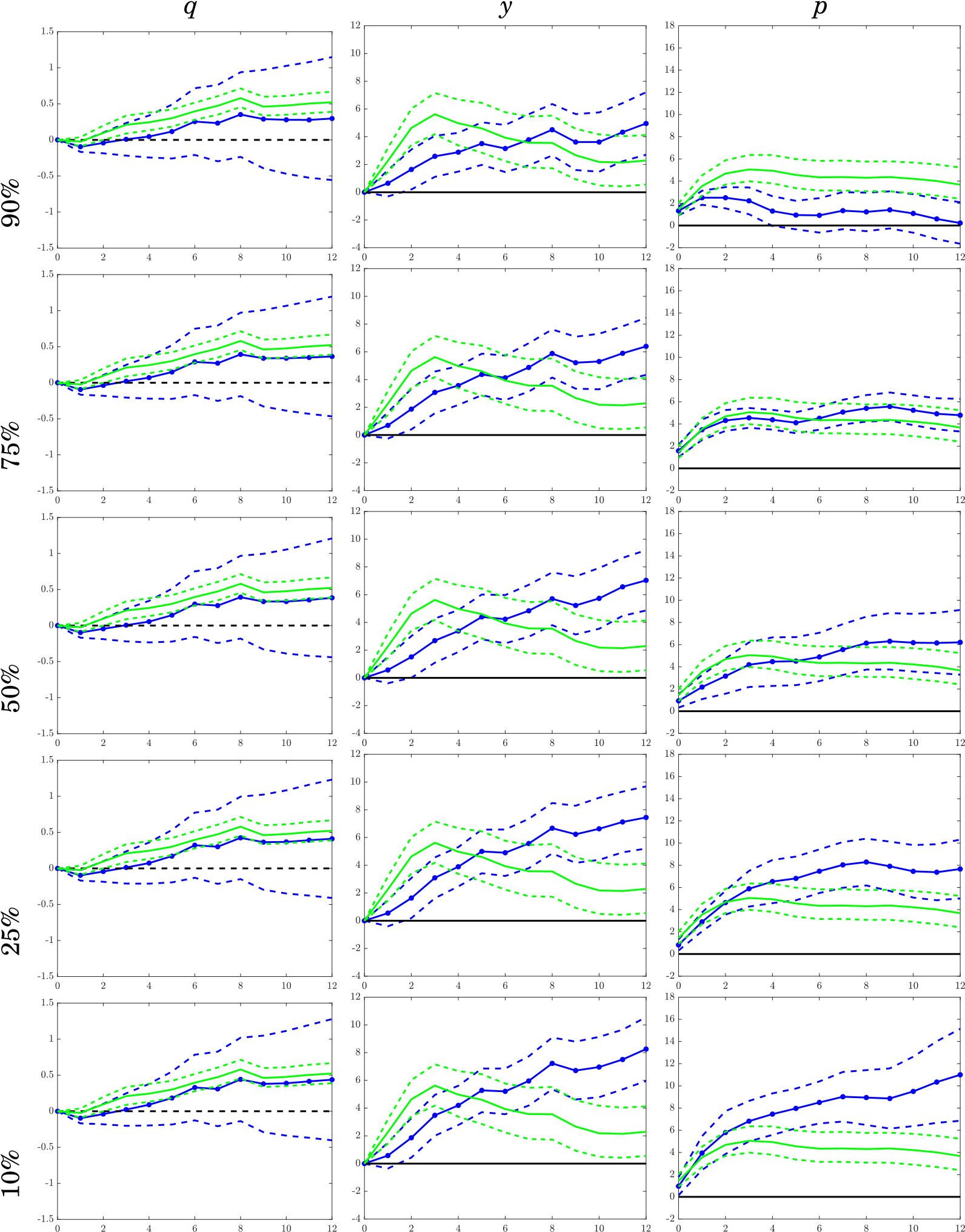
In this section, we present the empirical results from the quantile impulse response and forecast error variance decomposition. We first show the effect of unexpected business and consumer waves of optimism on the global oil market. The results are in Figures 1 and 2. In general, impulse responses were estimated while maintaining all the variables at the median quantile, but the real oil price was assumed to be held at the quantile of interest. Furthermore, we compared quantile results (blue lines) along with the ordinary least squares (OLS) at the mean (green lines).

Figure 1.Quantile Impulse Response BCI Shock

Note: This figure shows impulse response function from a shock from business expectations (bci) to oil production (q), real economic activity (y), and real oil price (p) (columns). Each row represent different quantiles for the real oil price. Blue lines are the quantile results and green lines are the mean-based results.

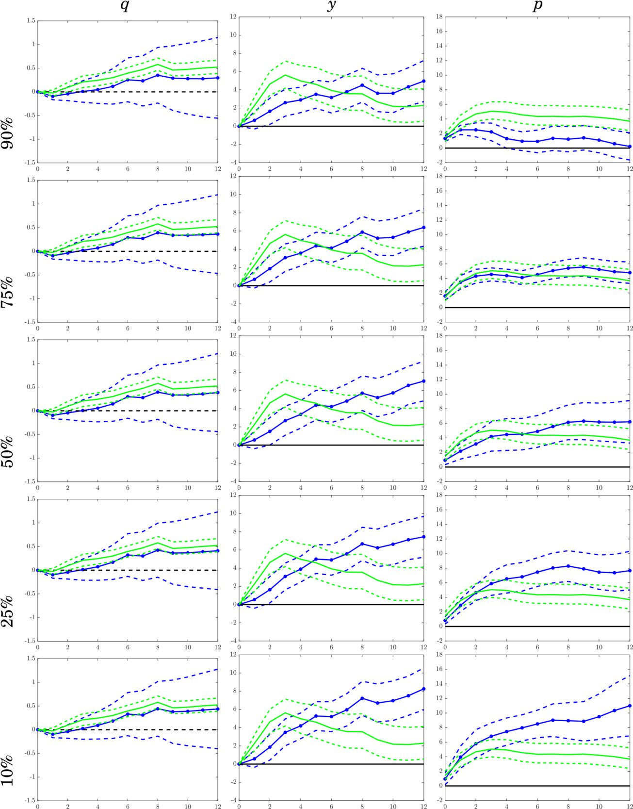
Figure 1 shows the results from an unexpected shock from businesses’ confidence to the three key variables in the global oil market model (columns). The rows represent the quantiles at which oil prices are estimated. As means of comparison, we also plotted the SVAR response in green. Similar to Byrne et al.'s (2019) findings, when an unexpected business expectation shock occurs, oil price initially increases for up to 3 months before a gradual decrease sets in. However, in the case of quantile impulse response (blue lines), business expectation shocks affect the entire oil price distribution differently. Specifically, oil price response is larger and more persistent at lower oil price quantiles.

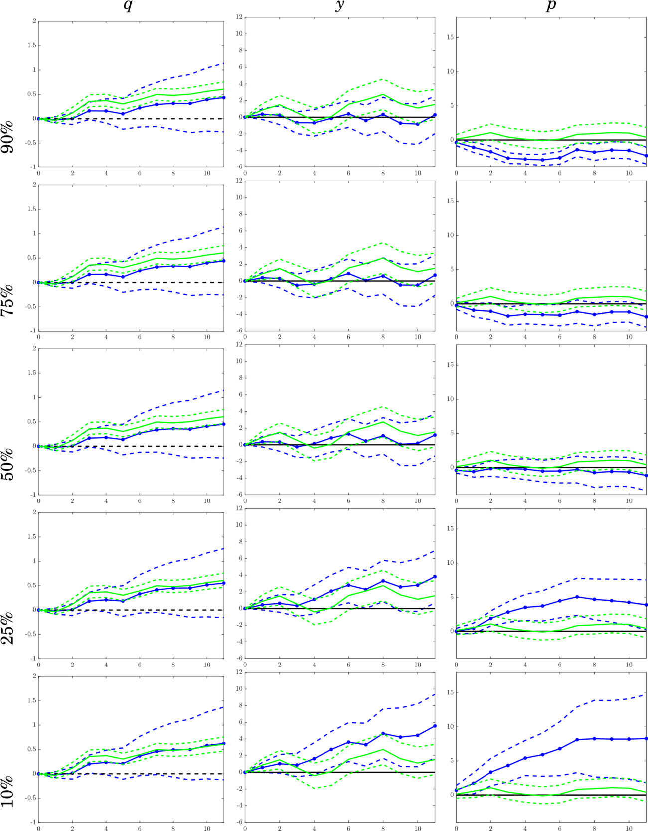
Concerning consumer expectations, Figure 2 shows the quantile impulse response results for the global oil market variables. Prior research does not attach much importance to the role of consumer expectations in oil price movements. In the mean-based SVAR literature (e.g., Byrne et al., 2019), represented by the green lines in Figure 2, since consumer expectations did not seem to affect the global demand for commodities, oil prices were not ultimately affected. Our results, represented by the blue lines, confirm this but with a slight but crucial modification. Consumer expectations affect oil prices significantly only at lower oil price quantiles. Therefore, when oil prices are low, an increase in consumer expectations would stimulate the global demand enough for commodities to increase oil prices from its mean value.

Figure 2.Quantile Impulse Response CCI Shock

Note. This figure shows impulse response function from a shock from consumer’s expectations (cci) to oil production (q), real economic activity (y), and real oil price (p) (columns). Each row represent different quantiles. Blue lines are the quantile results and green lines are the mean-based results.

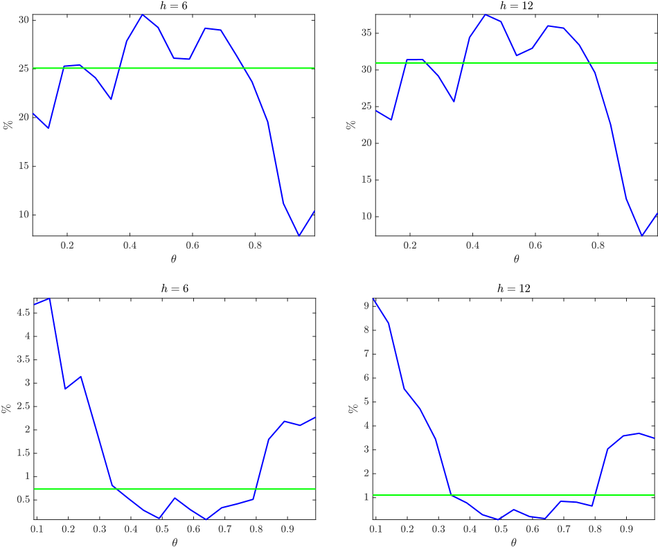
Furthermore, we carried out the forecast error variance decompositions (FEVD) from expectational shocks to the real oil price. Figure 3 shows the results for different forecast horizons (h = 6,12). The first and second rows present the BCI and CCI results, respectively. For each figure, the horizontal axis shows the FEVD at different real oil price quantiles, while the vertical axis shows the proportion of the variance attributed to the expectational variable. The blue lines show the QSVAR results, and the green lines show the mean-based OLS results.

Our results indicate that expectations make significant contributions to oil price variations across different oil price quantiles. The first row of Figure 3 shows that shocks to expectations from business leaders accounts for about 35% of the variance in oil prices. However, the contribution of this shock is highly quantile dependent. Business expectation shocks account for a large part of the forecast variance when oil prices are less than the 0.8 quantile. Subsequently, its importance decreases to about 10%. These results align with the impulse response evidence in Figure 1.

For consumer expectations (see the second row of Figure 3), the results are different. For 6 and 12 months, expectation shocks account for 0.73% and 1.11%, respectively, using the OLS approach (green line). The QSVAR results (blue line) are similar around the median (θ between 0.3 and 0.8). However, consumer expectation shock accounts for a larger fraction of oil price variability when oil price is at lower and higher quantiles. Furthermore, when oil prices are at their lowest quantiles, consumer confidence shocks can account for about 9% of total price fluctuation. As with business expectations, expectation shocks can have important asymmetric effects.

Figure 3.Forecast Error Variance Decomposition from BCI and CCI

Note: This Figure shows the FEVD from expectation shocks to oil price at different horizons (h= 6,12). The first row show the results bci and, second row, for cci. In each graph, blue and green lines represent the variance decomposition for QSVAR and OLS, respectively. Horizontal and vertical axes show the quantile and percentages of the variance, respectively.

IV. Conclusions

This study delved into the impact of innovations in businesses and consumer expectations regarding oil prices within a conventional global oil market model. We utilized a QSVAR model to dissect the complete response of oil price distribution following an expectation shock.

Our study revealed that the influence of expectations on oil prices varies across different quantiles. In line with existing literature, we confirmed the substantial impact of business expectations across the entire impulse response of oil price distribution. However, the magnitude and persistence vary according to the region of the distribution in which oil prices fall. Furthermore, contrary to prior research, we found that consumer expectations also play a pivotal role, especially when oil prices are at lower quantiles.

In summary, our findings suggest that in the absence of a direct connection between oil prices and fundamentals, expectations mostly influence oil price movements. Moreover, our results offer policymakers valuable insights into how expectations impact oil prices at varying quantiles. For higher oil price quantiles, policies targeting expectation management should focus on business expectations. Conversely, for lower oil price quantiles, similar policies should be directed toward managing consumer expectations.

Acknowledgement

The authors acknowledge insightful comments and suggestions from an anonymous reviewer and editor of this journal.

Funding

This work was partially funded by the Office of Research of the Universidad Católica de la Santísima Concepción through the Project DINREG 01/2022.